Perovskite Solar Cell (PSC) Tutorial Part A: Quick start - simulate your first perovskite device

🎯 Learning objectives

Run your first perovskite simulation in OghmaNano.
Generate and interpret a JV curve (J_SC, V_OC, FF, η).
Understand light JV curves

📦 Prerequisites

OghmaNano installed and working.
Basic familiarity with solar-cell concepts.

⏱ Estimated time

Part A: 5-10 min
Part B: 10-15 min
Part C: 15-20 min
Part D: 15-20 min
Part E: 10-15 min
Part F: 10-15 min
In total around an 1 hr depending on much you explore.

Crystal structure of a perovskite lattice showing the ABX₃ arrangement of atoms — The crystal structure of a perovskite (ABX₃) lattice. Large spheres represent the A-site cations, medium spheres the B-site cations, and small spheres the X-site anions. This simple cubic arrangement is the basis for the remarkable optoelectronic properties of perovskite solar cells.

Perovskite solar cells are one of the fastest-growing research topics in photovoltaics, with more than 30,000 publications since their breakthrough around 2012. Their rapid rise is driven by record power conversion efficiencies above 25%, placing them alongside crystalline silicon as leading solar technologies. At the same time, perovskites are uniquely challenging: issues such as ionic migration, hysteresis, and dynamic structural changes make them harder to fully understand than conventional semiconductors.

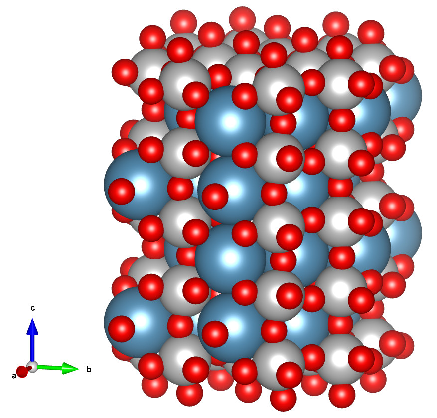
This tutorial uses a standard and widely studied structure – FTO / TiO₂ / MAPbI₃ (??) / Spiro-OMeTAD / Au – to introduce the fundamentals of perovskite solar cell simulation in OghmaNano. In just a few steps, you will launch the software, build the device stack, run a JV sweep, and analyse key results such as J_sc, V_oc, fill factor, and efficiency. Once you are comfortable with this basic device, the examples library includes more advanced perovskite systems and blends for further exploration.

Step 1: Launch OghmaNano

Start OghmaNano from the Windows Start menu. The main OghmaNano window will appear as shown in ??.

OghmaNano start window with options to create a new simulation, open a project, or access recent files — The OghmaNano start window. Create a new simulation, open an existing project, or access recent files.

Step 2: Create a new simulation

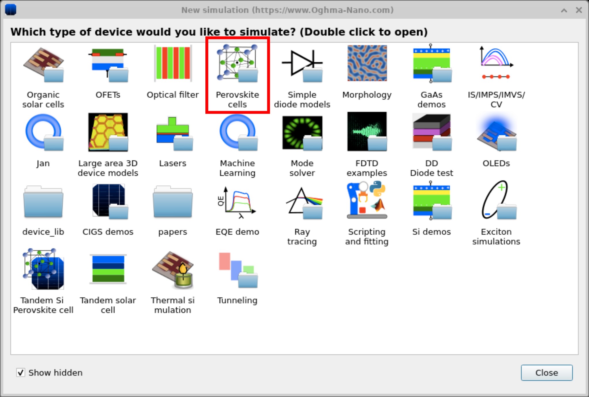
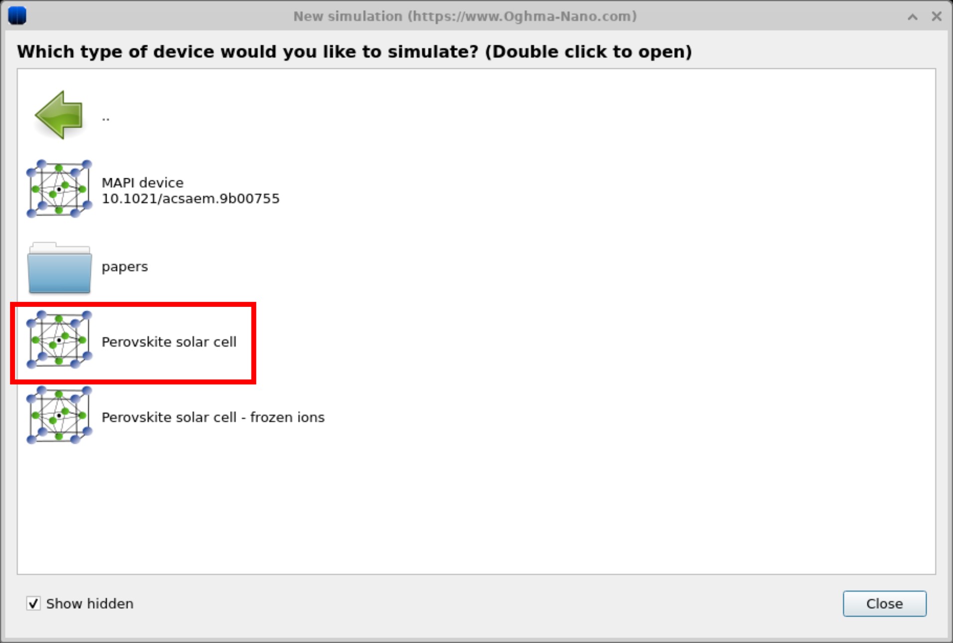
Click New simulation. This opens the library of available device types, shown in ??. Double-click Perovskite cells (highlighted in red) to open the perovskite examples folder. You’ll see a list of pre-set simulations, such as MAPbI₃ device and Perovskite solar cell, as shown in ??. For this tutorial, select the Perovskite solar cell template. When prompted, save the simulation to a folder you have write access to.

💡 Tip: For best performance save to a local drive such as C:\. Simulations stored on network, USB, or cloud folders (e.g. OneDrive) can run slowly due to heavy read/writes.

OghmaNano new simulation window with device categories including perovskite cells, OLEDs, OFETs, GaAs demos, ray tracing, and FDTD examples — The *New simulation* window provides a library of device types and example projects. Double-clicking a category opens preconfigured simulations — for example, the **Perovskite cells** folder highlighted here.

OghmaNano perovskite solar cell examples list showing preconfigured MAPbI₃ device and Perovskite solar cell templates — Within the *Perovskite cells* category you can choose from several pre-built device structures, including **MAPbI₃** and a generic **Perovskite solar cell**. These templates provide ready-to-run simulations that you can adapt to explore how material parameters and layer stacks affect performance.

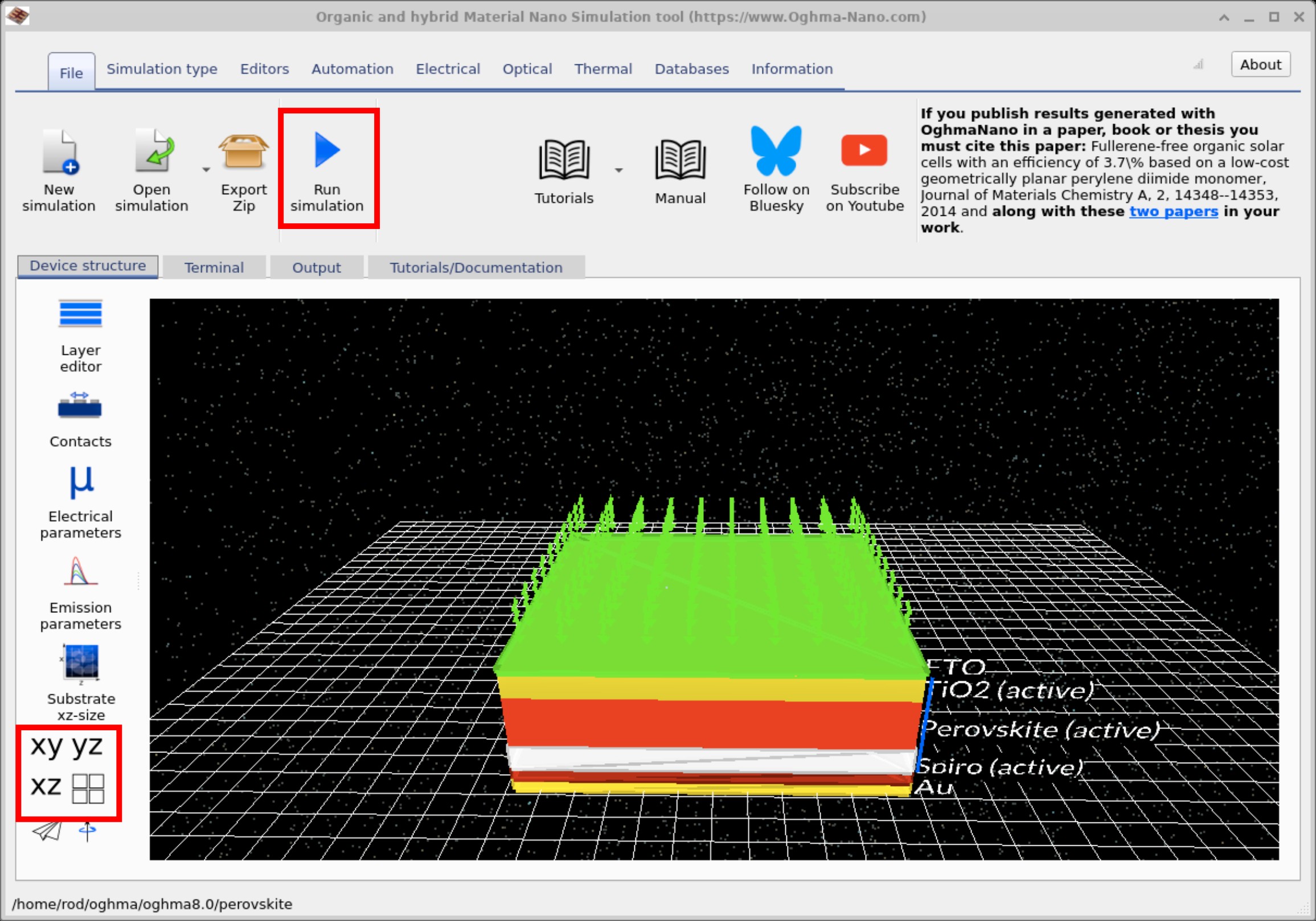
Step 3: Run the simulation

After selecting the template, the main simulation window opens (see ??). To start, click Run simulation (blue play icon) or press F9. Depending on your machine, the calculation may take a few seconds to complete. You can also use the xy / yz / xz buttons (bottom left) to change the device orientation in the 3D view.

Main OghmaNano interface showing the Run Simulation button and a 3D cross-section of a perovskite solar cell stack with layers labelled FTO, TiO₂, Perovskite, Spiro, and Au. — The main *OghmaNano* simulation interface. The toolbar provides quick access to common actions such as creating/opening simulations, exporting results, and running the solver. The 3D device view displays the stack of layers, here **FTO / TiO₂ / Perovskite / Spiro / Au**. Click the highlighted **Run Simulation** button (or press `F9`) to begin the calculation.

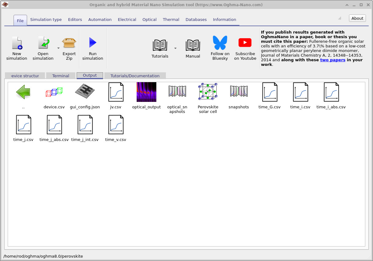
OghmaNano Output tab showing the working directory with simulation result files such as jv.csv, optical_output, snapshots, and time-dependent current/voltage data. — The *Output* tab of *OghmaNano*. Here you can browse the working directory for the current simulation. Typical results include `jv.csv` (JV curve data), `optical_output` (optical field results), `snapshots` (time-dependent fields), and time-resolved CSV files (`time_j.csv`, `time_v.csv`, etc.). Double-click any file to open it in the appropriate viewer or editor.

Step 4: View the results

Current density–voltage (JV) curve of a perovskite solar cell. The plot shows Jsc, Voc, and Pmax marked with arrows. — Example current density–voltage (JV) curve of a perovskite solar cell. *J_sc* (short-circuit current density) is the current at zero voltage. *V_oc* (open-circuit voltage) is the voltage at which the current density falls to zero. *P_max* marks the operating point where the product of current density and voltage is maximized, corresponding to the maximum power output of the device.

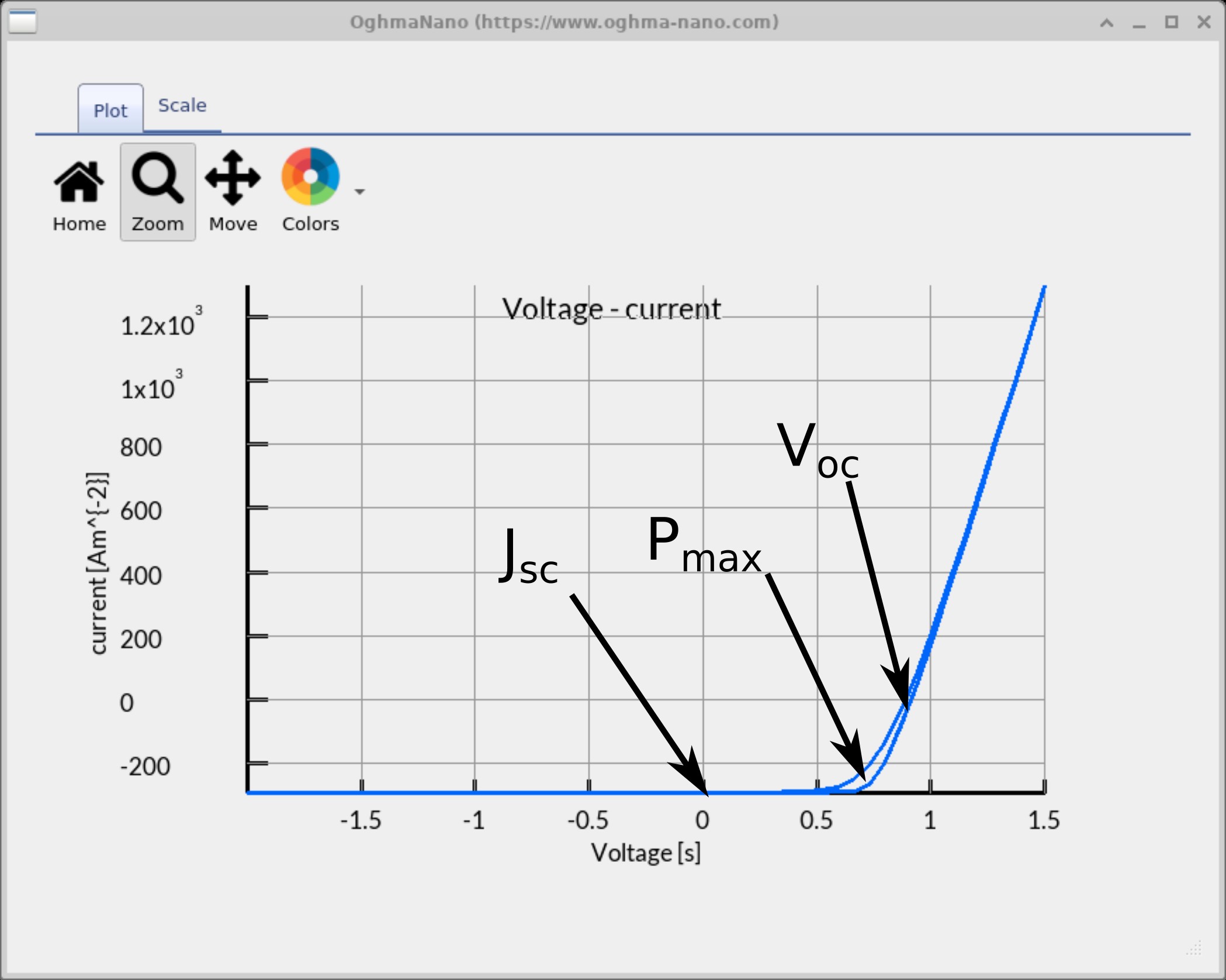
Open the Output tab (??) to browse the files written to disk. Double-click jv.csv to plot the JV curve (see ??). You can press g in the plot window to toggle the grid display. When examining the JV curve, focus on the following features (marked on the plot):

J_SC – the short-circuit current density, read where the curve crosses the current axis (V = 0). This shows how much current the cell produces without an external bias.
V_OC – the open-circuit voltage, where the curve crosses the voltage axis (J = 0). This is the maximum voltage the device can deliver under illumination.
P_max – the operating point (voltage × current) where the device produces maximum power.

Together, these parameters form some of the standard figures of merit for solar cells.

Well done! You’ve just run your first perovskite simulation and plotted its JV curve 🎉

💡 Show answer

This JV curve shows clear signs of hysteresis — it effectively contains two overlapping JV traces depending on whether the scan is taken in the forward or reverse direction. In perovskite solar cells, this arises because mobile ions (such as iodide vacancies) drift under an applied electric field. These ions redistribute during a voltage sweep, altering the local electric fields and charge extraction pathways. The result is a time-dependent response of the device, which manifests as hysteresis in the JV curve.

💡 Show answer

In perovskite solar cells, hysteresis can make it very difficult to define standard parameters such as the maximum power point, the open-circuit voltage, the short-circuit current, and even the fill factor. The JV curve may look different depending on the scan direction, scan speed, and device history, which complicates comparisons between results and makes reproducibility a key challenge in perovskite research.

Step 5: Changing the simulation mode to steady state

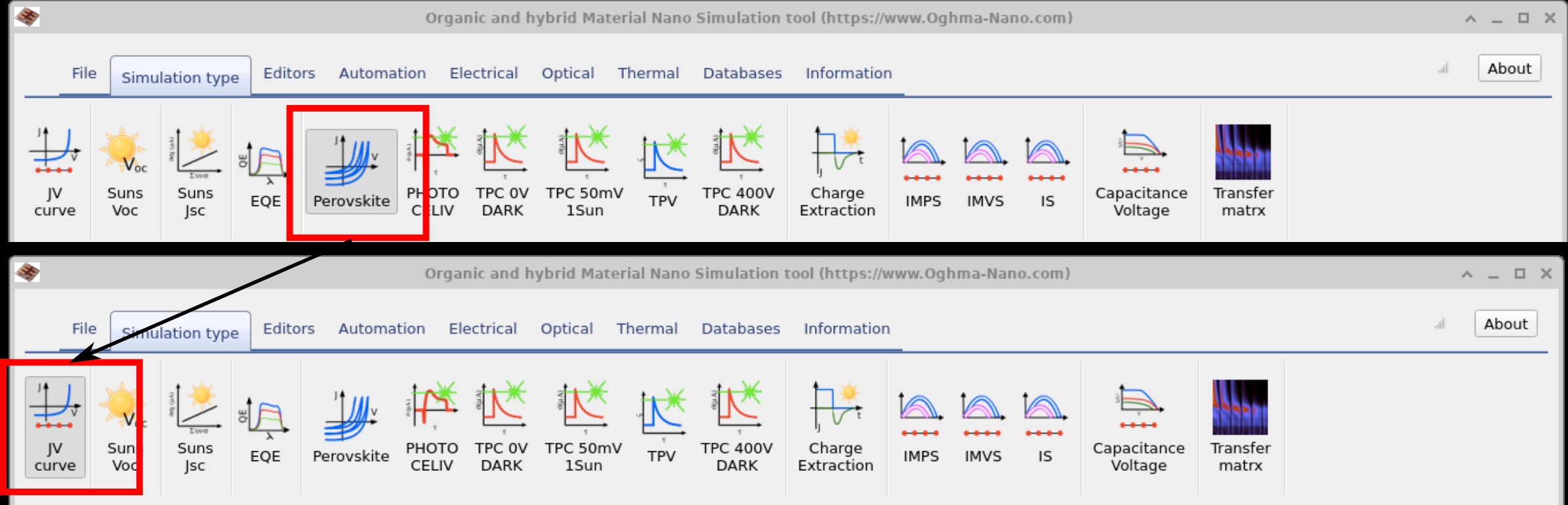
OghmaNano Simulation type ribbon highlighting how to switch from Perovskite (time-domain) to JV curve (steady-state) mode. — Switching to **steady-state**: In the *Simulation type* tab select **JV curve** to run a steady-state JV without hysteresis.

In the simulation above we ran the simulation in Hysteresis mode, which is a time-domain simulation. This mode accounts for how the applied potential redistributes mobile ions in perovskites over time. We swept the voltage from low to high and then back again, and—as you saw in the JV plot—the forward and reverse scans did not coincide because of this ionic motion (hysteresis). As noted above in the question boxes, such hysteresis makes it difficult to define stable values for PCE, J_SC, V_OC, and P_max, since they can depend on the device’s prior state. For the remainder of this tutorial we will disable hysteresis and run in steady-state mode. To do this, go to the Simulation type tab in the main OghmaNano window and click JV curve (see ??).

✅ What to expect

In steady-state mode the JV plot should now appear as a single, smooth sweep (no forward/reverse overlap). Note the values of J_sc, V_oc, FF, and PCE and compare them with the earlier hysteresis run to see how ionic effects impacted the metrics.

Step 6: The output from your simulation

Table 1: Files produced by the JV simulation
File name	Description
jv.csv	Current density vs voltage (JV curve)
charge.csv	Charge density vs voltage
device.dat	3D device model
fit_data*.inp	Experimental data for the example device (when provided)
k.csv	Recombination parameter vs voltage
reflect.csv / transmit.csv	Optical reflectance / transmittance
snapshots/	Electrical snapshots (bias/time dependent); see ??
optical_snapshots/	Optical field/intensity snapshots; see ??
sim_info.dat	Summary (V_OC, J_SC, FF, η); see ??
cache/	Intermediate cached data; see ??

Each simulation produces a collection of outputs that capture different aspects of device behaviour - from raw JV curves and charge densities, to optical spectra, recombination constants, and snapshots of electrical or optical fields. These files are usually plain csv files which can be opened directly in OghmaNano’s built-in viewers or processed externally (for example, plotting data in Excel or Python). The most important outputs for a basic perovskite study are summarised in Table 1 below.

👉 Next step: Now continue to Part B for a more detailed perovskite tutorial, including outputs, device layers, and advanced analysis.