Organic Solar Cell (OPV) Tutorial Part A: Quick start - simulate your first OPV device

🎯 Learning objectives

Run your first OPV simulation in OghmaNano.
Generate and interpret a JV curve (J_SC, V_OC, FF, η).
Understand light JV curves

📦 Prerequisites

OghmaNano installed and working.
Basic familiarity with solar-cell concepts.

⏱ Estimated time

Part A: 5-10 min
Part B: 10-15 min
Part C: 15-20 min
Part D: 15-20 min
Part E: 10-15 min
Part F: 10-15 min
In total around an 1 hr depending on much you explore.

Organic solar cells (OPVs) are the simplest device class in OghmaNano. They provide a straightforward way to learn the basics without dealing with 2D effects, ion migration, or light emission. In just a few steps, you’ll launch OghmaNano, set up a P3HT:PCBM device, run a JV sweep, and analyse the results. The examples library also includes other OPV material systems (e.g. PM6:Y6, D18:L8-BO) that you can explore once you’re comfortable with this simple material system - often described as the “fruit fly” of OPV research.

Step 1: Launch OghmaNano

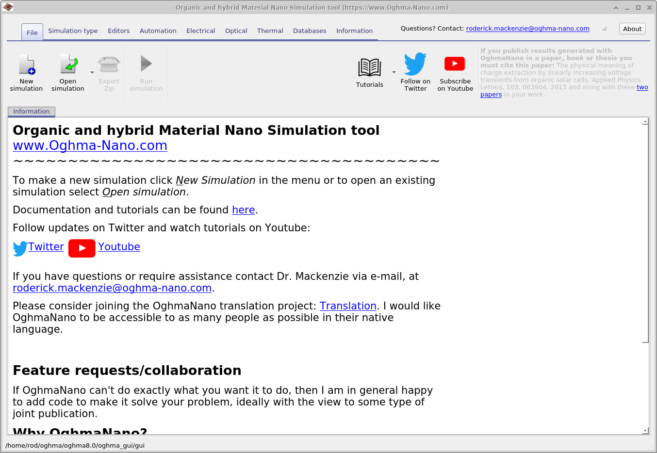
Start OghmaNano from the Windows Start menu. The main OghmaNano window will appear as shown in ??.

OghmaNano start window with options to create a new simulation, open a project, or access recent files — The OghmaNano start window. Create a new simulation, open an existing project, or access recent files.

Step 2: Create a new simulation

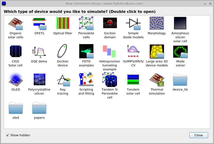
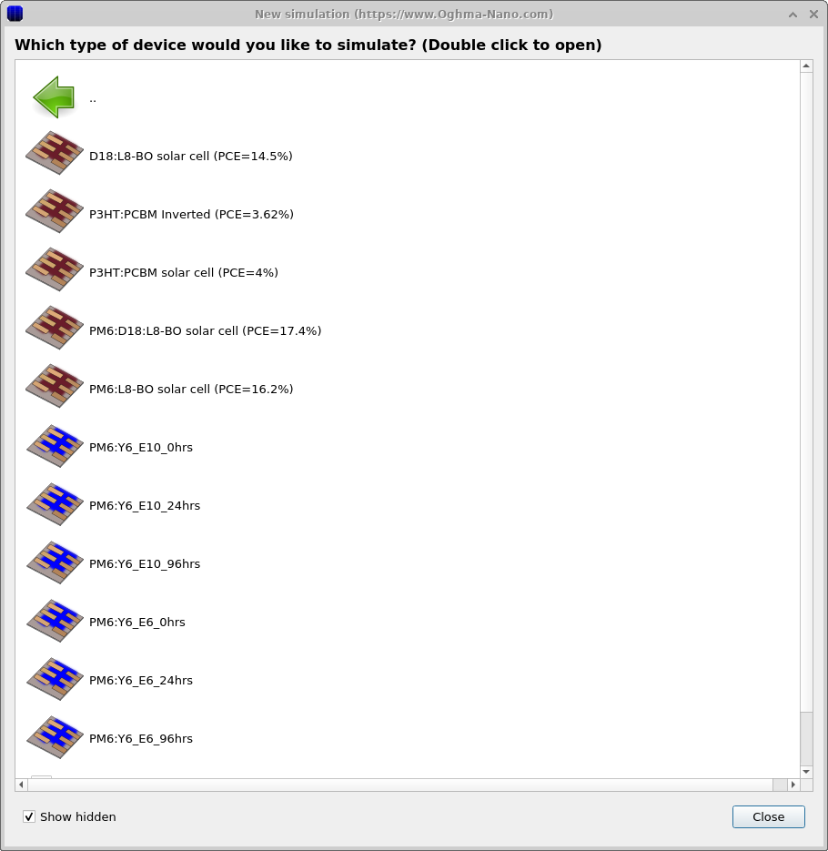
Click New simulation. This opens the library of available device types, shown in ??. Double-click Organic solar cells (top-left icon) to open the OPV examples folder. You’ll see a list of pre-set simulations such as P3HT:PCBM solar cell (PCE ≈ 4%), PM6:Y6, or D18:L8-BO, as shown in ??. For this tutorial, select the P3HT:PCBM solar cell (PCE = 4%). When prompted, save the simulation to a folder you have write access to.

💡 Tip: For best performance save to a local drive such as C:\. Simulations stored on network, USB, or cloud folders (e.g. OneDrive) can run slowly due to heavy read/writes.

OghmaNano new simulation window listing device categories such as organic solar cells, OLEDs, OFETs, perovskites, ray tracing, and FDTD examples — The *New simulation* window provides a library of device types and example projects. Double-click an icon to open a preconfigured simulation, such as organic solar cells, OLEDs, OFETs, perovskite cells, ray-tracing setups, or FDTD examples. These templates make it easy to explore different device classes without having to build each simulation from scratch.

OghmaNano organic solar cell examples list showing devices such as P3HT:PCBM, PM6:Y6, and D18:L8-BO with power conversion efficiencies — Within the *Organic solar cells* category you can choose from a range of pre-built OPV device structures. Each entry corresponds to a published or representative architecture (e.g. P3HT:PCBM, PM6:Y6, D18:L8-BO), with typical efficiencies noted in brackets. Double-clicking one of these templates opens a ready-to-run simulation that you can modify, helping you explore how active-layer materials and device stacks affect performance.

Step 3: Run the simulation

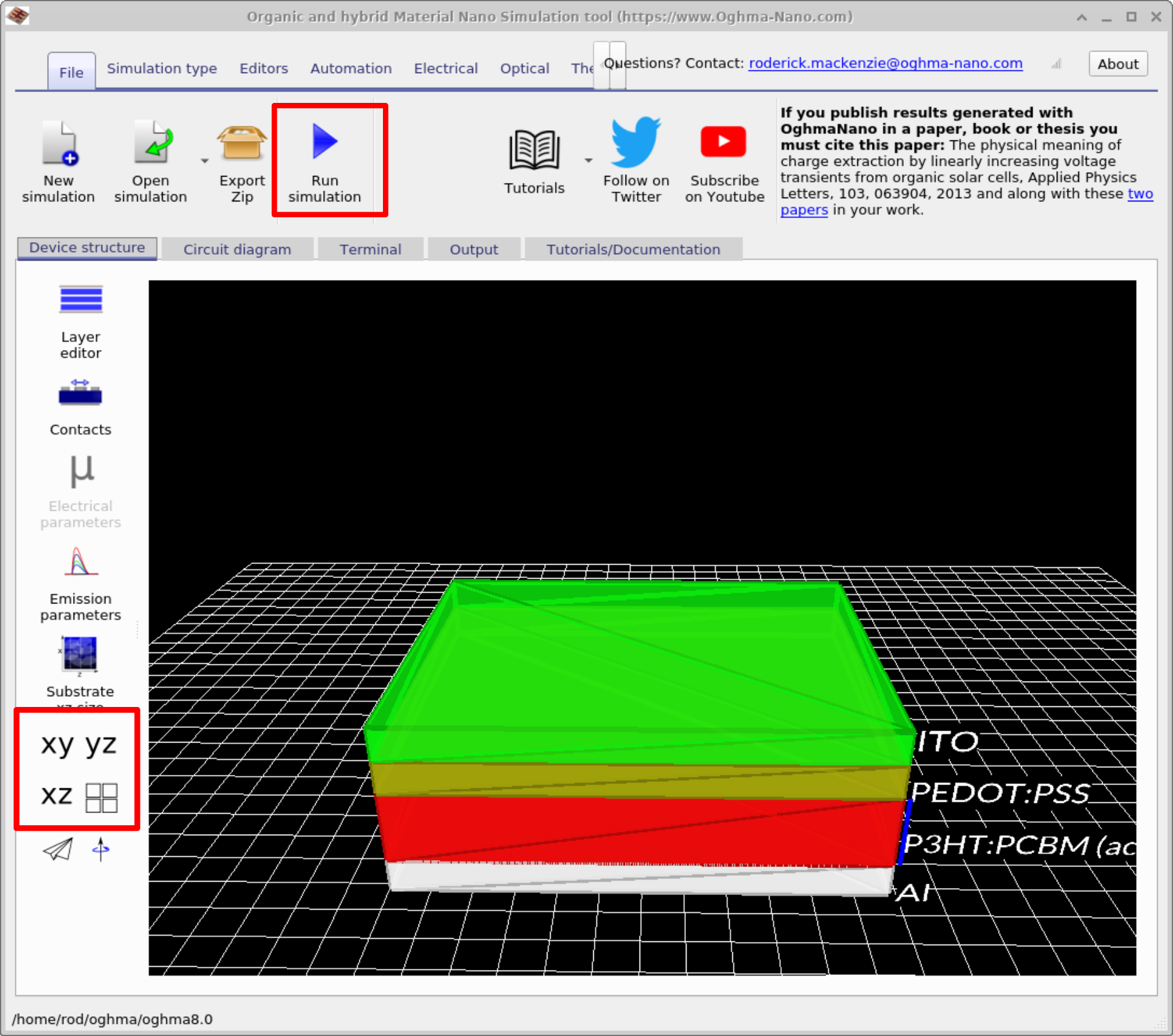
The main window opens (see ??). Click Run simulation (blue play icon) or press F9. On slower machines this may take a little while. Use the xy/yz/xz buttons to orient the device view.

Main OghmaNano interface showing the Run Simulation button and a 3D cross-section of a solar cell stack with layers labelled ITO, PEDOT:PSS, P3HT:PCBM, and Al. — The main *OghmaNano* simulation interface. The toolbar at the top provides quick access to actions such as creating or opening simulations, exporting, and running the solver. In the 3D panel the device stack is shown, with layers including ITO, PEDOT:PSS, the P3HT:PCBM active layer, and aluminium (Al) as the back contact. The highlighted **Run Simulation** button (or `F9`) starts the calculation.

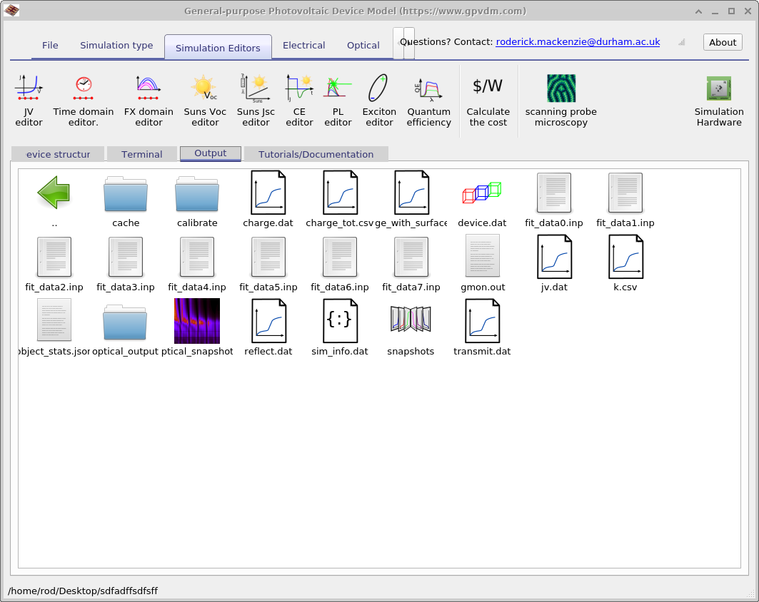
OghmaNano Output tab displaying the simulation working directory with result files such as jv.csv, reflect.dat, snapshots, and input files. — The *Output* tab of *OghmaNano*. This view exposes the working directory for the current simulation, showing generated result files such as `jv.dat` (JV curve data), `reflect.dat` (reflection spectrum), `snapshots` (optical/electrical field profiles), and the various input parameter files. Double-clicking a file opens it in the appropriate viewer or editor.

Step 4: View the results

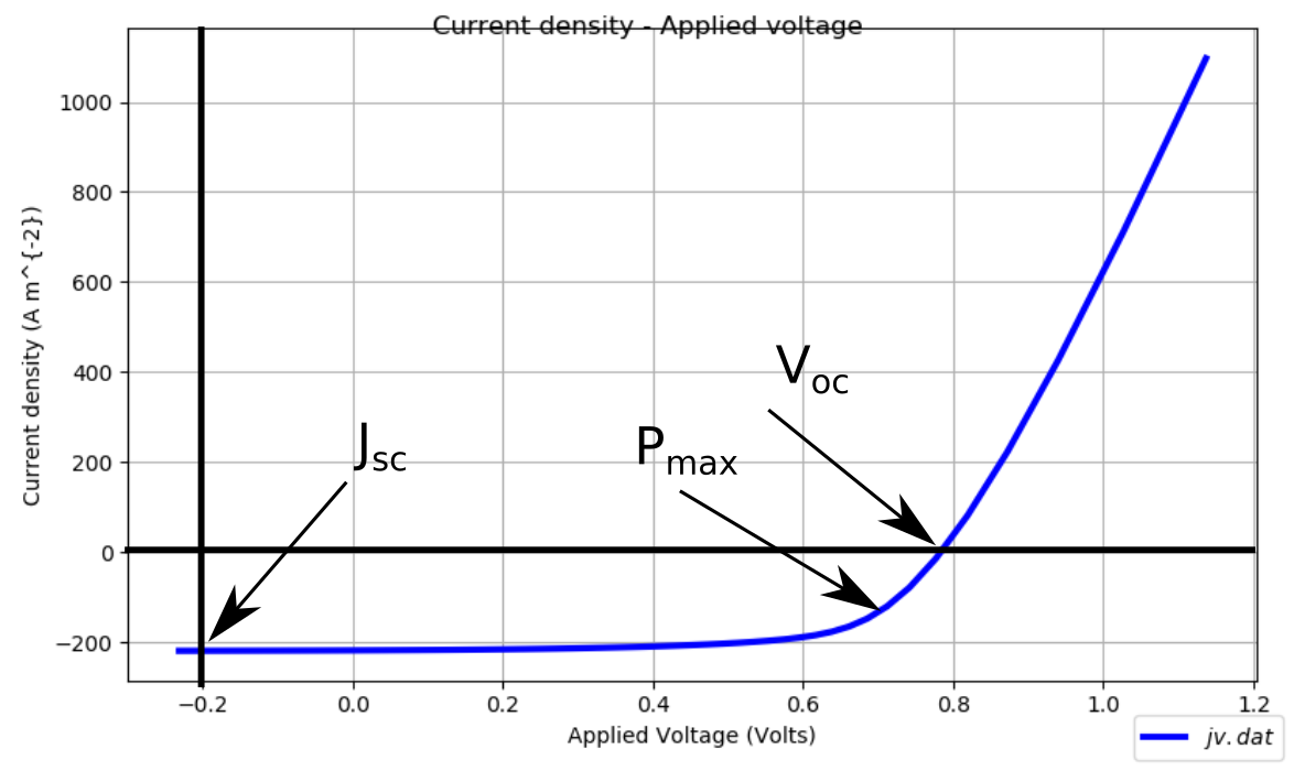
Open the Output tab (see Figure 7) to browse files written to disk. Open jv.dat to view the JV curve (see Figure 6). Press g in the plot window to toggle a grid. When examining the JV curve, focus on the following features (marked on the plot):

J_SC - the short-circuit current density, read where the curve crosses the current axis (V = 0). This tells you how much current the cell produces under illumination without an external voltage.
V_OC - the open-circuit voltage, found where the curve crosses the voltage axis (J = 0). This is the maximum voltage the device can deliver under light.
P_max - the operating point (voltage × current) at which the device produces maximum power.

Together, these parameters form some of the standard figures of merit for solar cells.

Current density–voltage (JV) curve of an organic solar cell. The curve shows Jsc at negative bias, Voc at the zero-current intercept, and Pmax at the knee of the curve. — Example current density–voltage (JV) curve of an organic solar cell. *J_sc* (short-circuit current density) is the current at zero applied voltage. *V_oc* (open-circuit voltage) is the voltage at which the current density falls to zero. *P_max* marks the operating point where the product of current density and voltage is maximized, corresponding to the maximum power output of the device.

Nice! You’ve run your first OPV simulation and plotted its JV curve.

The output from your simulation

Each simulation produces a collection of outputs that capture different aspects of device behaviour - from raw JV curves and charge densities, to optical spectra, recombination constants, and snapshots of electrical or optical fields. These files are usually plain csv files which can be opened directly in OghmaNano’s built-in viewers or processed externally (for example, plotting data in Excel or Python). The most important outputs for a basic OPV study are summarised in Table 1 below.

Table 1: Files produced by the JV simulation
File name	Description
jv.csv	Current density vs voltage (JV curve)
charge.csv	Charge density vs voltage
device.dat	3D device model
fit_data*.inp	Experimental data for the example device (when provided)
k.csv	Recombination parameter vs voltage
reflect.csv / transmit.csv	Optical reflectance / transmittance
snapshots/	Electrical snapshots (bias/time dependent); see ??
optical_snapshots/	Optical field/intensity snapshots; see ??
sim_info.dat	Summary (V_OC, J_SC, FF, η); see ??
cache/	Intermediate cached data; see ??

👉 Next step: Now continue to Part B for a more detailed OPV tutorial, including outputs, device layers, and advanced analysis.