

Organic Tandem Solar Cell Simulation: PCDTBT:PC70BM / PM6:Y6 and Cross-Interface Recombination
1. Introduction: why combine two organic solar cells?
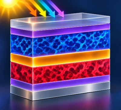
Organic photovoltaic absorbers offer chemically tuneable optical spectra and can be deposited as thin films. A tandem solar cell places two absorbers in the optical path so that the first intercepts part of the incident spectrum and the second uses photons transmitted through it. Here the front absorber is PCDTBT:PC70BM, while the rear absorber is PM6:Y6. These blends have different optical absorption characteristics and effective electrical gaps.
The example is a monolithic, two-terminal (2T) tandem. The subcells share one external current and their voltages contribute to the terminal voltage. An internal junction must allow electrons arriving from one subcell to recombine with holes arriving from the other. Rather than inserting a thin artificial recombination semiconductor, this example uses a cross-interface recombination boundary condition directly between the two absorber regions.
The electrical parameters are intentionally effective-medium values, suitable for demonstrating the coupled model rather than claiming a calibrated description of a particular fabricated device. The optical datasets and band parameters are treated separately.
2. Opening the organic tandem example
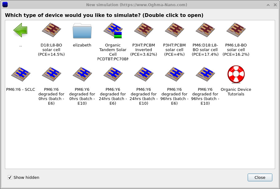
Start OghmaNano and select New simulation (??). Locate the organic tandem example in the simulation browser (??) and open it. The Device structure view (??) shows the complete optical stack.
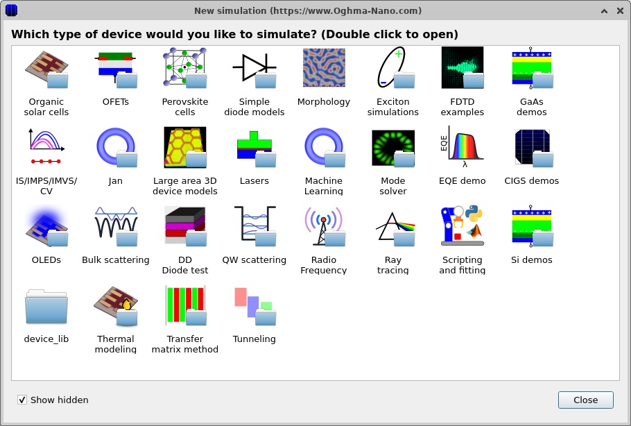
Save a copy before changing parameters. The Electrical ribbon contains the Layer, Contact, Interface and Electrical parameter editors (??).
3. Running the organic tandem solar-cell simulation
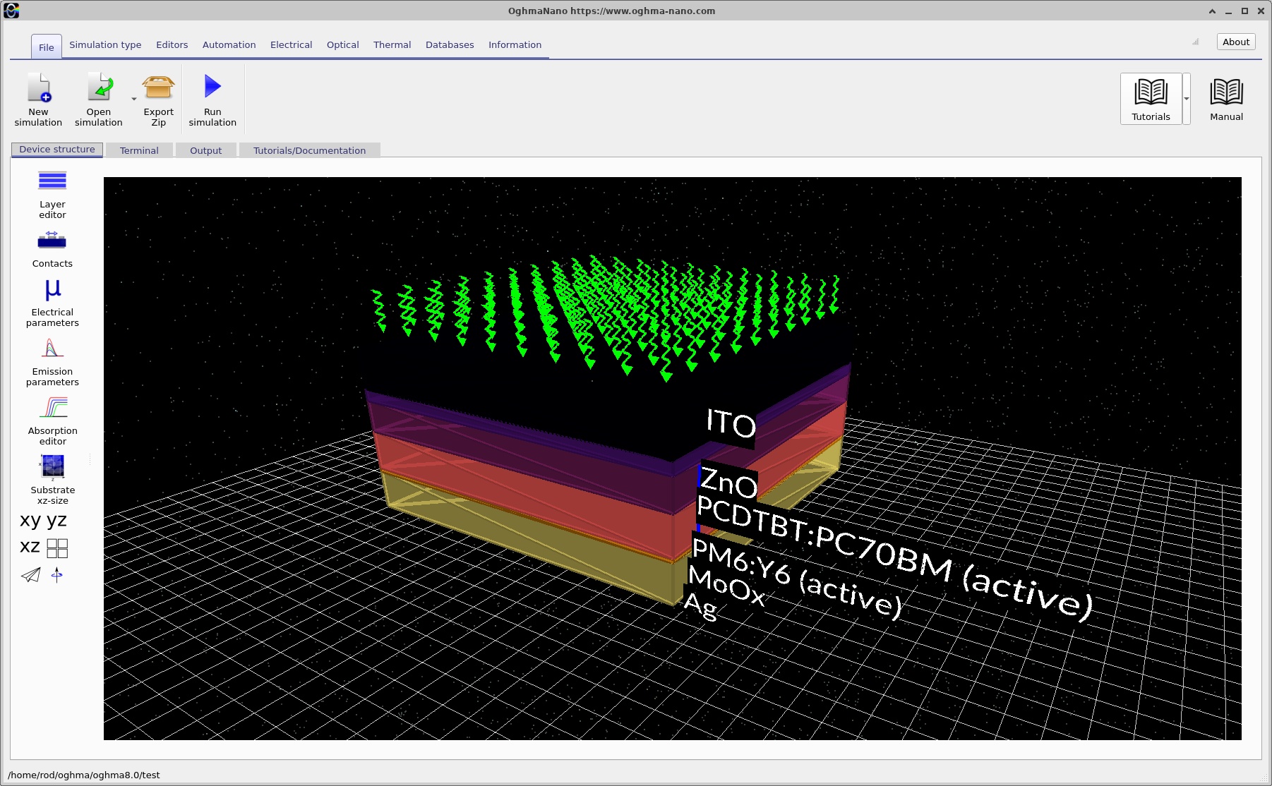
The three-dimensional representation of the organic tandem solar cell is shown in ??. The device contains two electrically active organic absorber layers, PCDTBT:PC70BM and PM6:Y6, positioned between the front and rear electrodes. The two absorbers are connected through a zero-thickness recombination interface, which provides the electrical connection between the subcells.
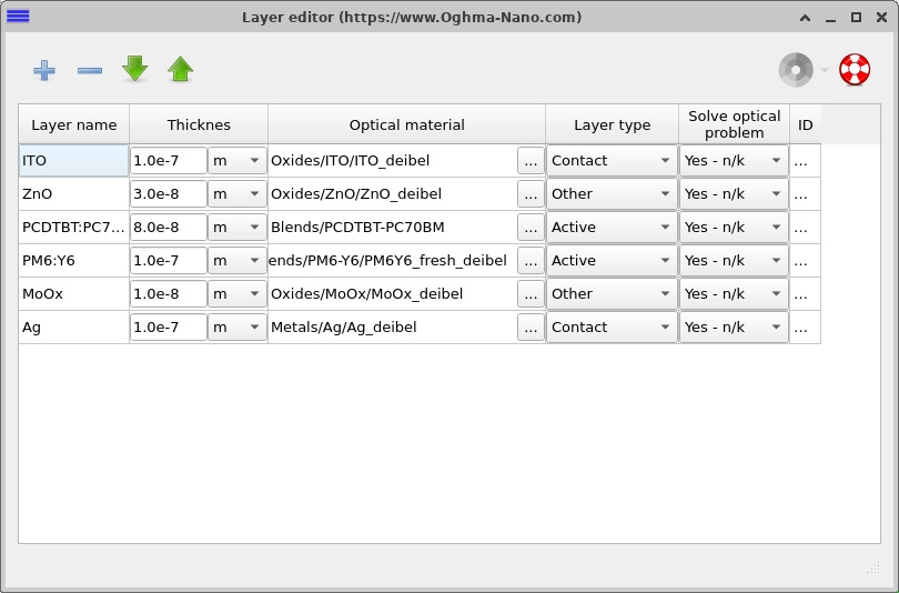
Click the Layers button in the Electrical ribbon to open the Layer editor, shown in ??. This window lists the materials, thicknesses and electrical configuration of each layer in the device.
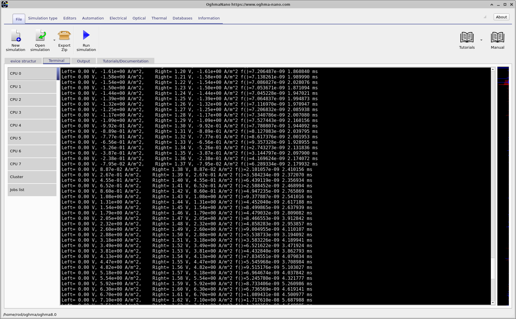
To run the simulation, click the blue Run simulation button or press F9. The numerical solver calculates the current-voltage (J-V) characteristic of the complete tandem device. The solver output is shown in ??. Notice that the current crosses zero at approximately 1.38 V, corresponding to the open-circuit voltage \(V_{OC}\) of the tandem solar cell.
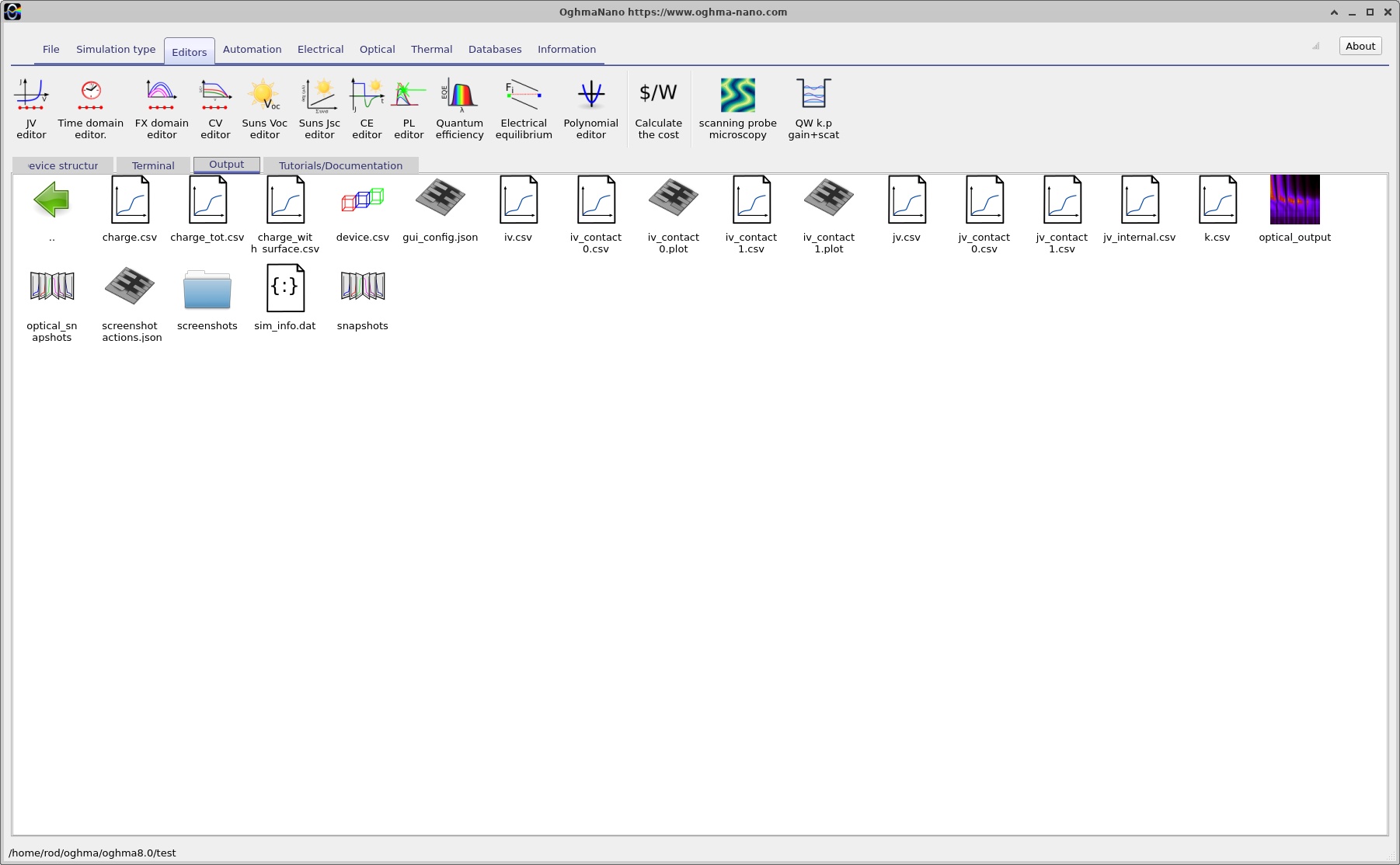
Once the calculation has finished, open the Output tab, shown in ??. This contains the files generated by the simulation, including the calculated J-V characteristic, internal carrier distributions and simulation information.
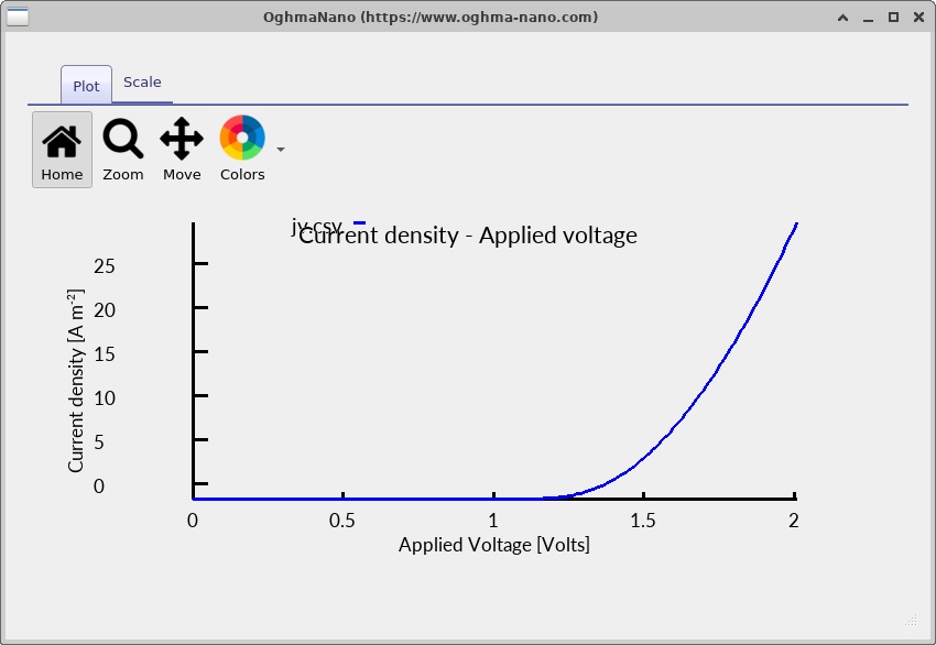
Double-click jv.csv to open the calculated current-voltage
characteristic
(??).
The two subcells are electrically connected in series, so they carry
the same current while their photovoltages contribute to the
total terminal voltage.
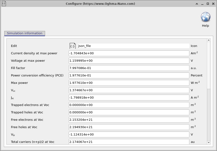
Double-click sim_info.dat to open the simulation information
(??).
This file contains information about the calculated device performance
and simulation settings.
jv.csv.
sim_info.dat.
The device consists of six layers, listed below from the illuminated front surface to the rear electrode. The ZnO and MoOx layers are included in the optical structure but are not separately resolved as electrically active semiconductor regions. The two organic absorber layers form the electrically active tandem structure.
| Layer (front to rear) | Thickness | Role |
|---|---|---|
| ITO | 100 nm | Transparent front electrode. |
| ZnO | 30 nm | Front optical/transport-layer material. |
| PCDTBT:PC70BM | 80 nm | Front organic bulk-heterojunction absorber with the larger effective electrical gap. |
| PM6:Y6 | 100 nm | Rear organic bulk-heterojunction absorber with the smaller effective electrical gap. |
| MoOx | 10 nm | Rear optical/transport-layer material. |
| Ag | 100 nm | Rear metal electrode. |
The recombination boundary lies directly between PCDTBT:PC70BM and PM6:Y6. It has zero geometrical thickness and therefore does not appear as an additional layer in the table. The cross-interface recombination mechanism is examined later in this tutorial.
Notice that the open-circuit voltage (\(V_{OC}\)) reported in ?? is approximately 1.37 V, considerably higher than would typically be expected from a single-junction organic solar cell. This illustrates one of the main advantages of a tandem structure: the photovoltages generated by the two subcells add together, producing a higher overall open-circuit voltage.
4. Electrical parameters and bulk recombination
The electrical properties of the two organic absorbers can be inspected by clicking the Electrical Parameters button in the main OghmaNano window. This opens the electrical parameter editor, where the material bandgaps, electron affinities, carrier mobilities, densities of states and recombination mechanisms can be configured. The parameter windows for PCDTBT:PC70BM and PM6:Y6 are shown in ?? and ??, respectively.
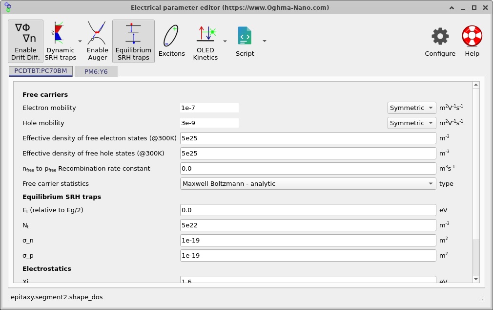
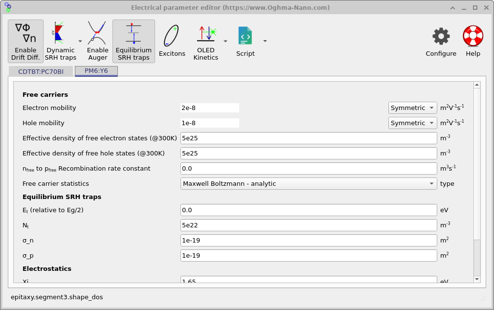
The example uses representative effective electrical parameters for the two organic bulk-heterojunction absorbers. The mobilities and densities of states are chosen to give physically reasonable charge-transport behaviour, while the bandgaps and electron affinities provide an illustrative energetic alignment between the subcells. These parameters describe an effective drift-diffusion model rather than the complete microscopic electronic structure of the individual donor and acceptor materials.
| Parameter | PCDTBT:PC70BM | PM6:Y6 |
|---|---|---|
| Effective electrical gap, Eg | 1.60 eV | 1.35 eV |
| Electron affinity, χ | 1.60 eV | 1.65 eV |
| Electron mobility, μn | 1 × 10⁻⁷ m² V−1 s−1 | 2 × 10⁻⁸ m² V−1 s−1 |
| Hole mobility, μp | 3 × 10⁻⁹ m² V−1 s−1 | 1 × 10⁻⁸ m² V−1 s−1 |
| Effective densities of states, Nc and Nv | 5 × 1025 m−3 | 5 × 1025 m−3 |
| Bulk recombination | Equilibrium SRH | Equilibrium SRH |
Charge trapping and trap-assisted recombination are particularly important in disordered organic semiconductors, where structural disorder, energetic defects and localised electronic states can strongly influence carrier transport and recombination. For this reason, the example uses Shockley–Read–Hall (SRH) recombination rather than a simple free-to-free bimolecular recombination model. SRH recombination provides a convenient effective description of recombination mediated by localised trap states, although other recombination mechanisms may also be important in real organic photovoltaic devices.
Both absorbers use the equilibrium SRH model with an effective trap density of 5 × 10²² m−3 and electron and hole capture cross sections of 10−19 m². In the conventional single-level approximation, the recombination rate is written as
\[ R_{\mathrm{SRH}} = \frac{np-n^{eq}p^{eq}} {\tau_p(n+n_1)+\tau_n(p+p_1)}. \]Here, \(n\) and \(p\) are the free electron and hole densities, \(n^{eq}\) and \(p^{eq}\) are their equilibrium values, \(\tau_n\) and \(\tau_p\) are the electron and hole capture lifetimes, and \(n_1\) and \(p_1\) describe the carrier concentrations associated with the trap energy. The recombination rate depends on the available carrier populations and vanishes at thermal equilibrium. This bulk recombination process is distinct from the cross-interface recombination mechanism used to connect the two photovoltaic subcells.
5. Modelling the Tandem Recombination Layer
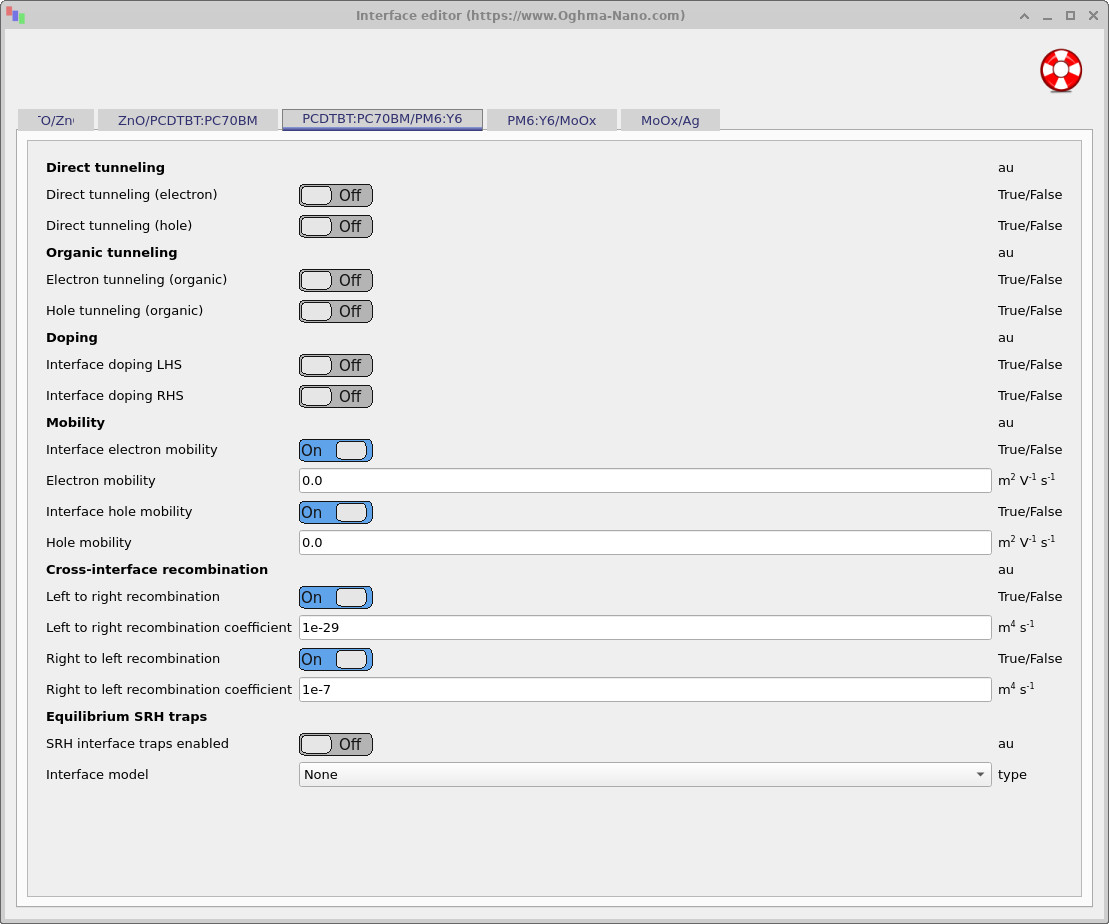
In this device, the recombination region between the two organic absorbers is represented by an infinitely thin interface. This interface allows electrons on one side to recombine directly with holes on the other, providing the electrical connection between the two photovoltaic subcells. Conventional electron and hole drift-diffusion transport across the interface is disabled, so the subcells are connected through the interfacial recombination mechanism rather than ordinary carrier transport across the boundary.
In a fabricated tandem solar cell, this function would normally be performed by an interconnection or recombination layer, often consisting of thin electron- and hole-selective transport layers together with a highly recombination-active contact, such as a thin metallic or conducting oxide interlayer. Rather than explicitly modelling these additional layers, their combined electrical function is represented by the boundary condition shown in ??.
To inspect the model, open the Interface editor and select the PCDTBT:PC70BM/PM6:Y6 interface. The electron and hole interface mobility overrides are enabled and set to zero, preventing ordinary drift and diffusion between the absorbers. The cross-interface recombination model is then used to connect the two subcells electrically.
The recombination mechanism removes an electron on one side of the interface and a hole on the other. The two possible carrier pairings are described by
\[ R_{l2r}=K_{l2r}\left(n_Lp_R-n_L^{eq}p_R^{eq}\right), \] \[ R_{r2l}=K_{r2l}\left(n_Rp_L-n_R^{eq}p_L^{eq}\right). \]Here, \(L\) and \(R\) denote the mesh points immediately to the left and right of the interface, while the superscript \(eq\) denotes equilibrium carrier concentrations. The coefficients \(K_{l2r}\) and \(K_{r2l}\) have units of m4 s−1, giving recombination rates per unit area in m−2 s−1. The corresponding recombination current density is \(J_{\mathrm{rec}}=qR\). Subtracting the equilibrium carrier product ensures that the net recombination rate vanishes at thermal equilibrium.
In this example, the dominant recombination pathway is between electrons in PM6:Y6 on the right and holes in PCDTBT:PC70BM on the left. The coefficients are \(K_{r2l}=10^{-7}\,\mathrm{m^4\,s^{-1}}\) and \(K_{l2r}=10^{-29}\,\mathrm{m^4\,s^{-1}}\). The large difference between these values makes the recombination strongly directional, as required by the arrangement of the two photovoltaic junctions.
The purpose of the recombination interface is to provide an electrically conducting connection between the subcells while allowing their individual photovoltages to add together. An efficient interconnection brings the relevant electron and hole quasi-Fermi levels close together at the centre of the device, minimising the voltage lost across the recombination junction.
Under Boltzmann statistics, the electron population on the right and the hole population on the left are related to their quasi-Fermi-level separation by
\[ n_Rp_L=n_R^{eq}p_L^{eq} \exp\left(\frac{E_{Fn,R}-E_{Fp,L}}{k_BT}\right). \]The recombination current can therefore be written as
\[ J_{\mathrm{rec}}= qK_{r2l}n_R^{eq}p_L^{eq} \left[ \exp\left(\frac{E_{Fn,R}-E_{Fp,L}}{k_BT}\right)-1 \right]. \]As the recombination coefficient increases, a smaller separation between \(E_{Fn,R}\) and \(E_{Fp,L}\) is needed to sustain the same current. In the strong-recombination limit, these two quasi-Fermi levels approach one another, creating an effective recombination contact between the subcells. This allows the photovoltage generated by each absorber to contribute to the overall tandem voltage, while reducing the voltage loss associated with the interconnection.
An alternative approach is to introduce an explicit thin recombination layer between the absorbers and assign it a very large bimolecular recombination coefficient,
\[ R=B\left(np-n^{eq}p^{eq}\right). \]Although this can produce a similar electrical connection, the combination of a very thin layer and an extremely high recombination rate can introduce additional mesh requirements and numerical stiffness, making the coupled drift-diffusion equations more difficult to converge. The zero-thickness cross-interface model avoids these additional degrees of freedom and provides a more direct and numerically efficient way to represent the interconnection when its internal structure does not need to be resolved.
For further details, see the semiconductor interface theory and the interface editor reference.
6. Contacts and the electrical mesh
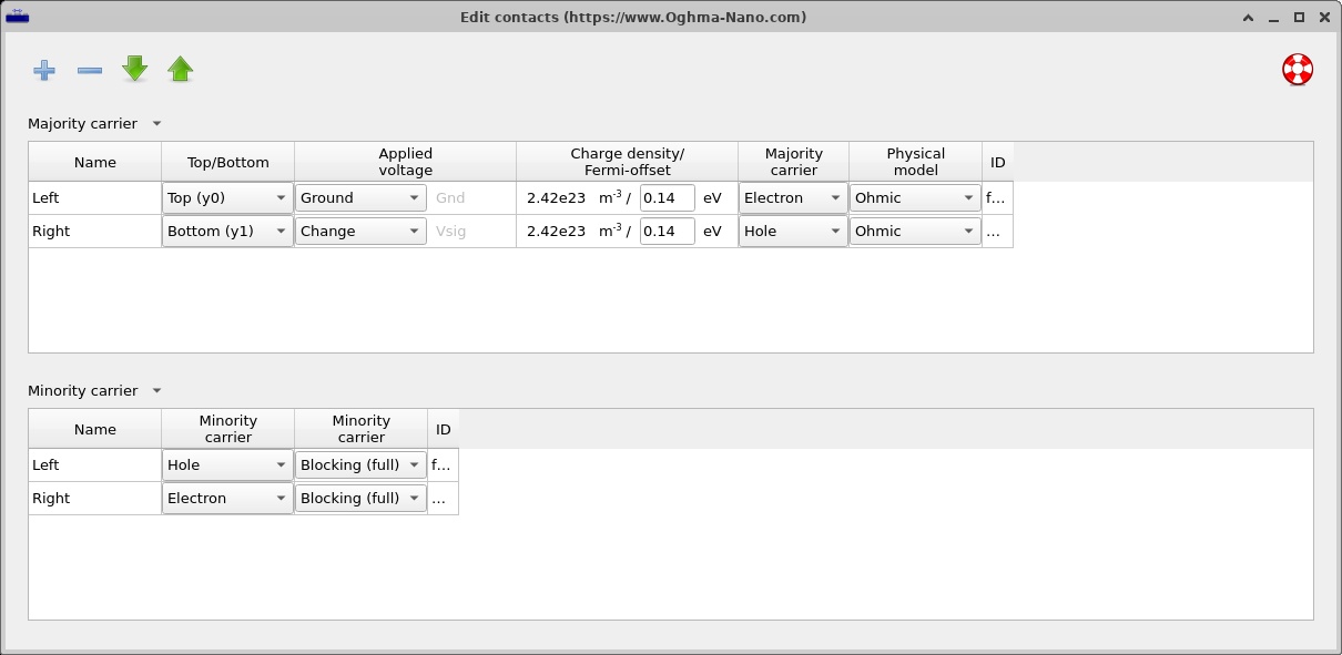
Inspect the two external contacts in the Contacts editor (??). The front boundary is grounded and electron-majority; the rear is the swept-voltage, hole-majority terminal. These electrical boundary conditions have been retained from the working model. The ZnO and MoOx layers remain in the optical structure, but the electrical calculation does not need them as separately solved selective layers.
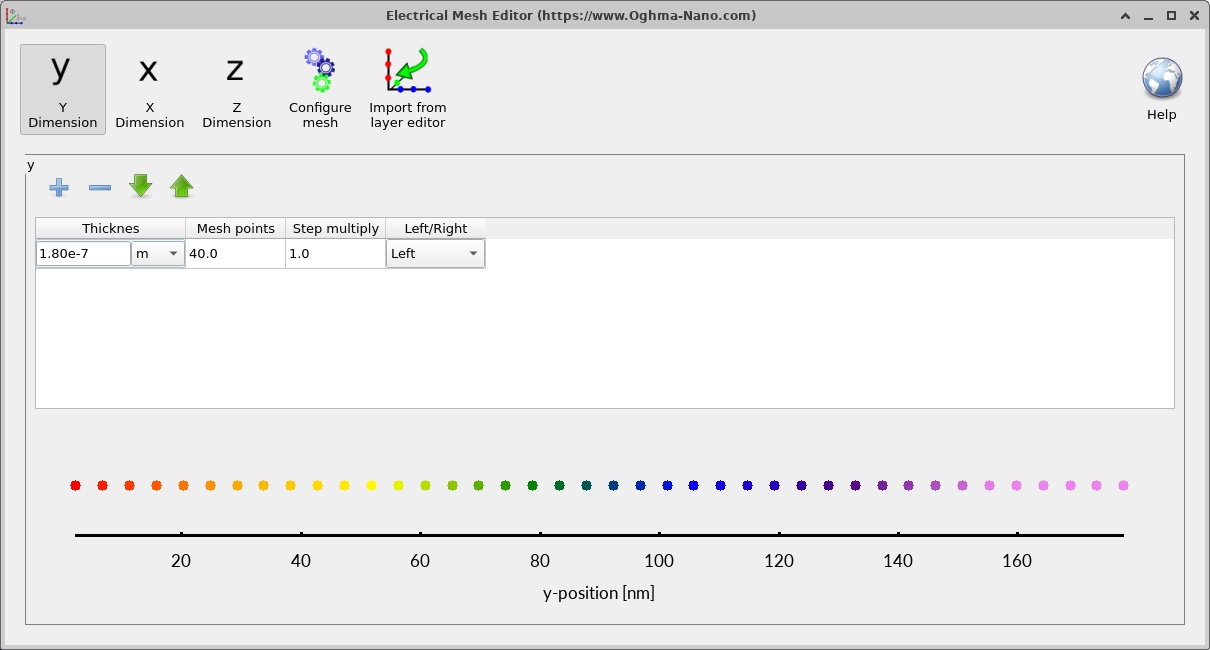
Next inspect the one-dimensional Electrical mesh (??). The two absorbers must meet at the correctly located material boundary so the solver can apply the cross-interface source/sink terms to the adjacent mesh points. There is no finite-thickness interlayer mesh to resolve.
For two subcells connected electrically in series, the current density is common to both subcells; it is not the sum of their separate photocurrents. A photovoltaic J-V curve is commonly characterised by its short-circuit current density, open-circuit voltage and maximum-power point, provided the simulated bias range includes these operating points.
\[FF=\frac{|J_{mpp}V_{mpp}|}{|J_{SC}|V_{OC}},\qquad \eta=\frac{|J_{mpp}V_{mpp}|}{P_{in}}.\]Interpret the shape and sign of the displayed J-V trace using the simulation's current convention. The plotted example demonstrates the coupled electrical response; it should not be treated as an experimentally calibrated efficiency claim. Check the underlying CSV before reporting numerical performance figures.
8. Band structure and quasi-Fermi levels
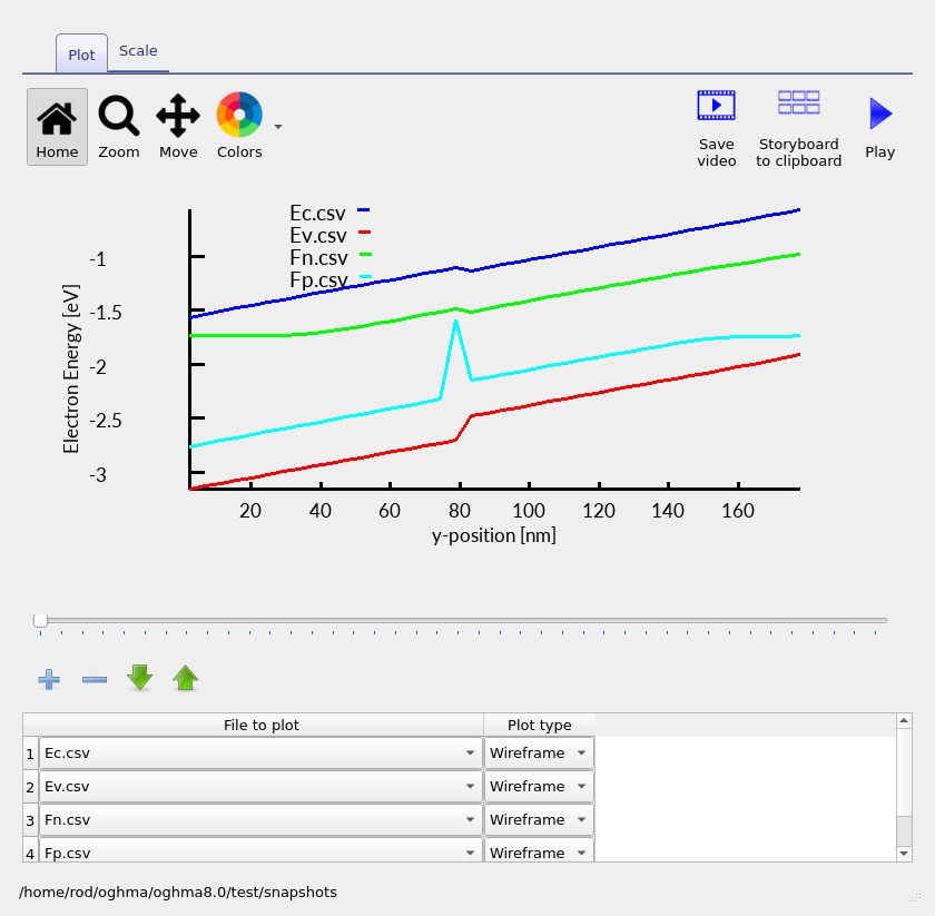
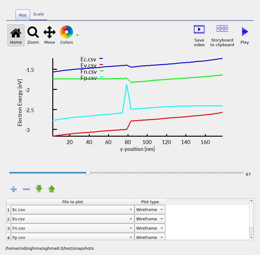
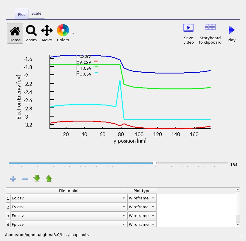
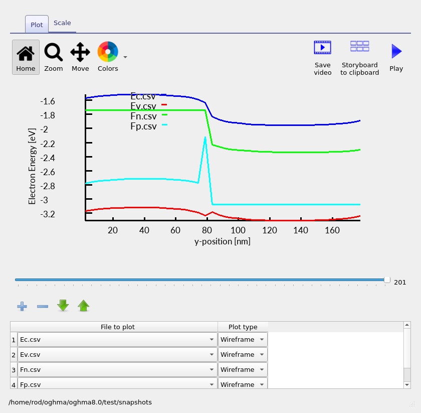
Open the saved band-structure plots and move through the stored voltage snapshots (??, ??, ?? and ??). The conduction and valence mobility edges reflect the effective gaps and affinities, while their spatial bending follows the self-consistent electrostatic potential.
Under illumination, the separation of electron and hole quasi-Fermi levels within each absorber expresses its local nonequilibrium carrier population. At the interconnection, the strong cross-interface rate tends to bring EFn,R and EFp,L closer together. This is the electrical signature of an effective recombination contact: finite current can pass through recombination with only a limited interconnection quasi-Fermi-level splitting.
9. Electron and hole current profiles
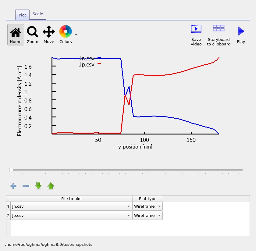
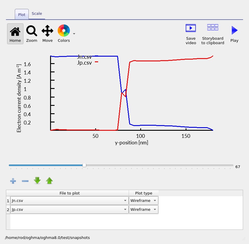
The electron and hole current plots are particularly informative for a tandem. Within either absorber, the partition between electron and hole current changes with position as carriers are generated, transported and recombine. At the central interface, conventional cross-boundary electron and hole drift–diffusion currents are suppressed by the zero mobility overrides.
Instead, the boundary condition consumes a hole from one subcell and an electron from the other. The interfacial recombination current therefore transfers the series connection between the two carrier channels. The current profiles (??–??) provide a direct way to see how the subcells remain electrically coupled without requiring individual carriers to drift through an artificial recombination layer.
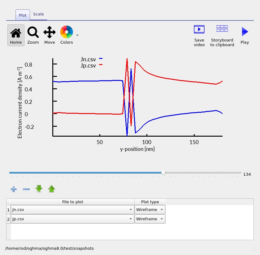
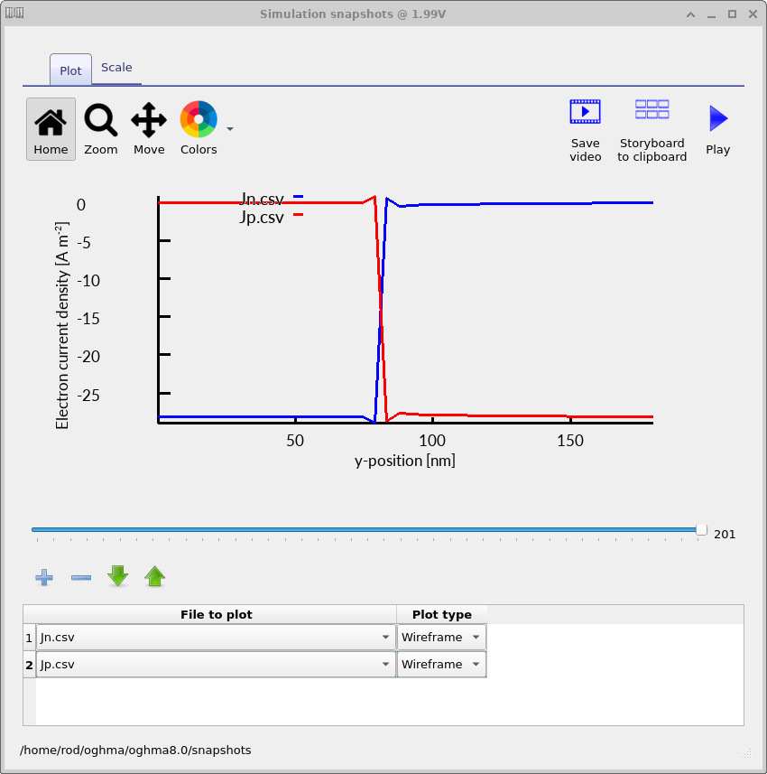
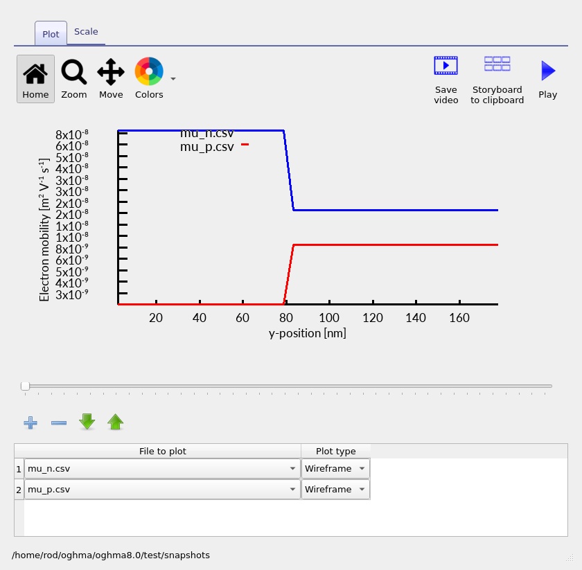
The profile of the spatially varying carrier mobility (??) helps distinguish ordinary transport within the bulk absorbers from the special boundary treatment at their interface. The zero face-mobility override applies only at the selected interface, not throughout either absorber.
10. Optical generation and transfer-matrix analysis
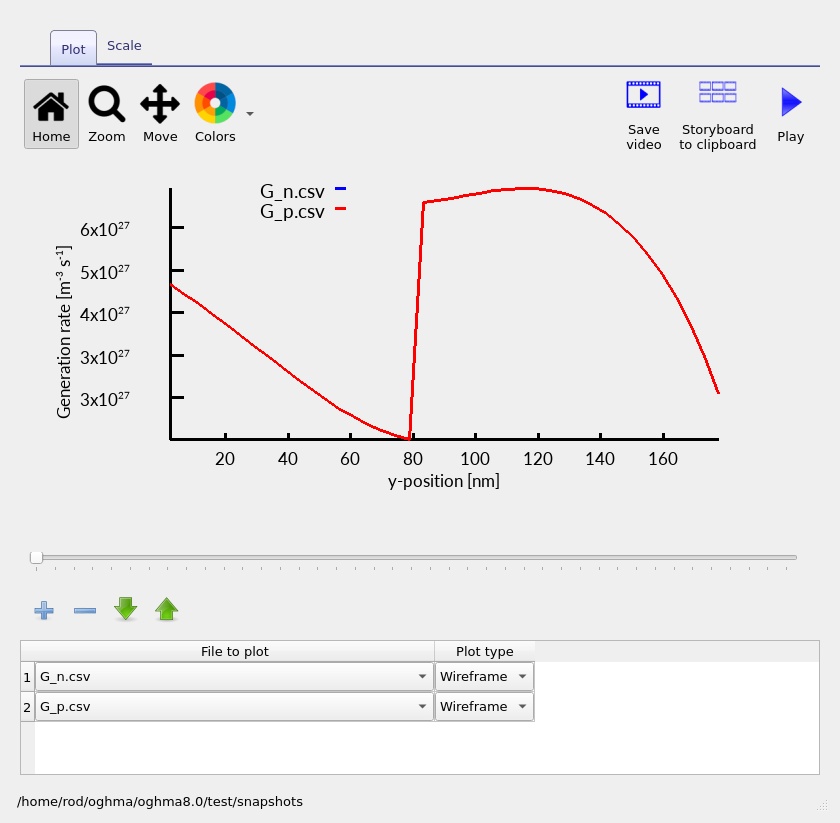
The organic blends have different absorption spectra, so the optical calculation determines both how much light enters each absorber and where photocarriers are generated. In the one-dimensional description,
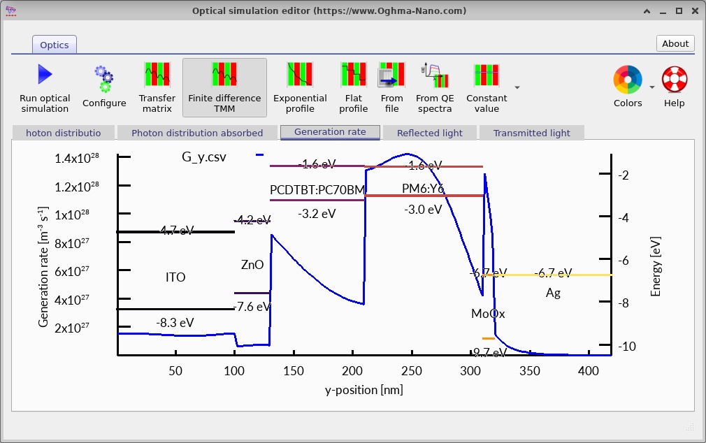
\[G(y)=\int\alpha(\lambda,y)\,\Phi(\lambda,y)\,d\lambda,\]where α is the local absorption coefficient and Φ is an appropriately defined spectral photon flux. The transfer-matrix model also includes interference and reflections in the multilayer optical stack.
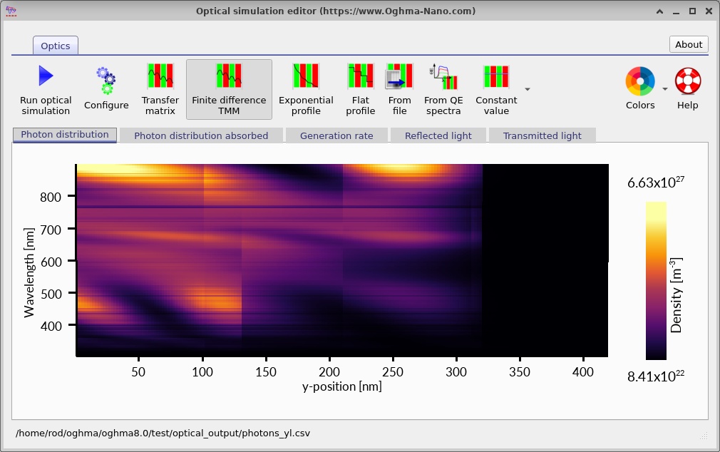
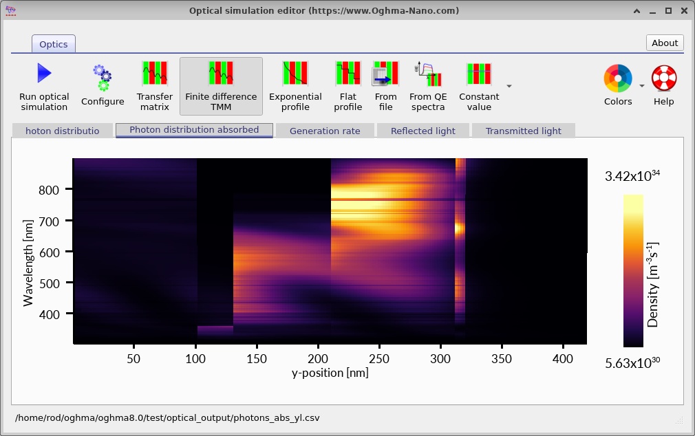
The spatial generation profile (??) shows where carriers are created. The two absorbers share the same incident optical stack but receive different local spectra because light is absorbed and reflected on its way through the device.
Explore the optical-analysis tabs (??, ?? and ??). They show complementary views of wavelength- and position-dependent optical response. The first cell may remove photons which would otherwise be available to the second, so increasing its thickness does not necessarily increase the total series-connected output.
11. Suns-Voc and Suns-Jsc
11.1. Suns-Voc
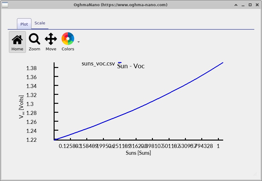
Select Suns-Voc to examine the terminal open-circuit voltage as the illumination level changes. Greater photogeneration generally increases the quasi-Fermi-level splitting in the subcells and hence the terminal voltage. A simple illuminated-diode approximation gives
\[V_{OC}\simeq\frac{n_{id}k_BT}{q}\ln\!\left(\frac{J_{ph}}{J_0}+1\right).\]In a tandem, the terminal voltage includes the contribution of both subcells and any loss in the recombination interconnection. The result is shown in ??.
11.2. Suns-Jsc
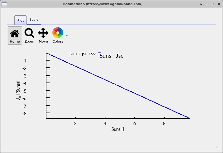
Run Suns-Jsc to follow the short-circuit current with illumination intensity. If collection remains approximately unchanged, the response is often close to linear, \(|J_{SC}|\propto P_{sun}\). Any deviation can reflect changes in recombination, charge collection or the operating balance of the two series-connected subcells.
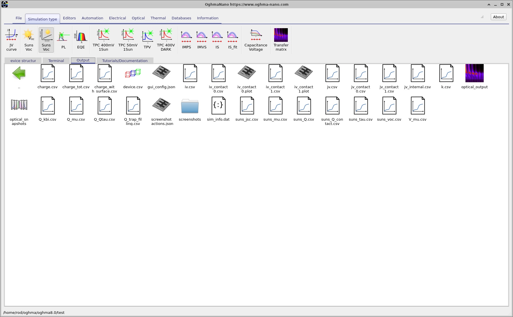
The output view and current trend are shown in ?? and ??.
12. Suggested investigations
The principal lesson is that optical stacking and electrical interconnection must be solved together. The front blend shapes the spectrum reaching the rear blend, while the zero-thickness recombination boundary couples their electron and hole transport without an artificial electrical interlayer.