OghmaNano contains an advanced three-dimensional ray-tracing solver for modelling optical systems, lenses, apertures, rough surfaces, microlenses, and structured optoelectronic assemblies. The ray-tracing module is designed for problems in imaging optics, optical filtering, surface scattering, light extraction, and geometric optical design. By combining explicit three-dimensional geometry with wavelength-dependent material properties, the solver allows users to analyse how light propagates through realistic optical components and complete assemblies.
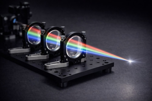
The same framework can be applied to a broad range of optical systems, including Cooke triplet lenses, long-focal-length prime lenses, general ray-tracing feature tours, reflection from rough films, light escape from structured films, and microlens and optical filtering demonstrations. Because the solver operates directly on traced rays through full three-dimensional geometry, it is particularly useful for studying focusing, aberrations, collection efficiency, detector response, and wavelength-dependent behaviour in optical systems that are too complex for simpler paraxial approximations.
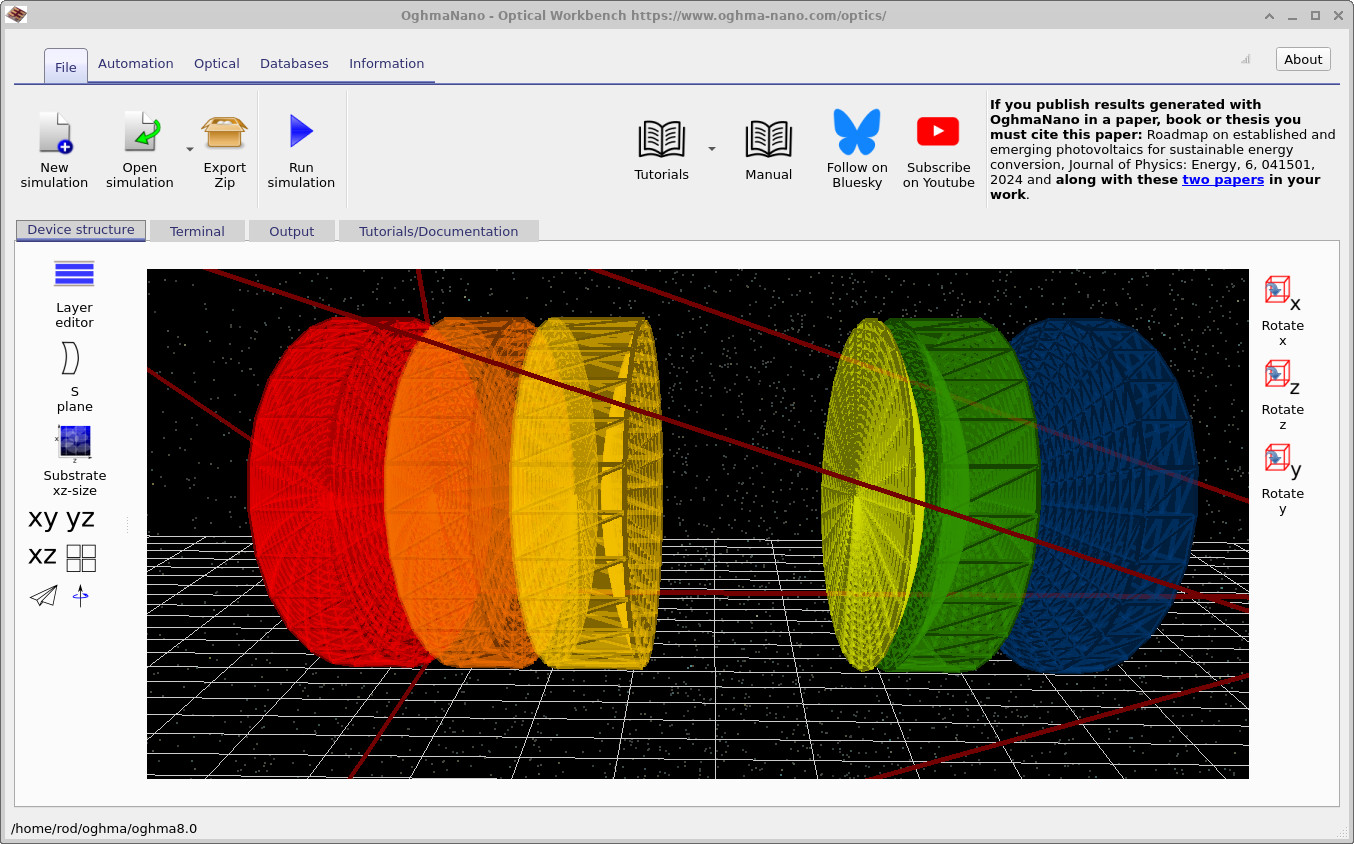
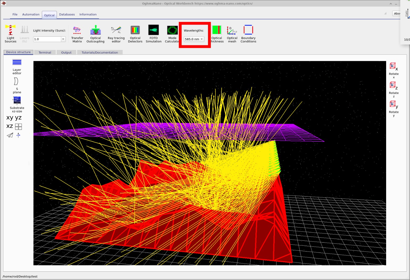
OghmaNano provides dedicated tools for defining light sources, placing optical detectors, and editing lens-based optical systems using the S-plane editor. In practice this allows users to move from a compact lens prescription to a full three-dimensional scene, trace rays across wavelength, and analyse both the geometry and the resulting detector-plane image within one workflow.
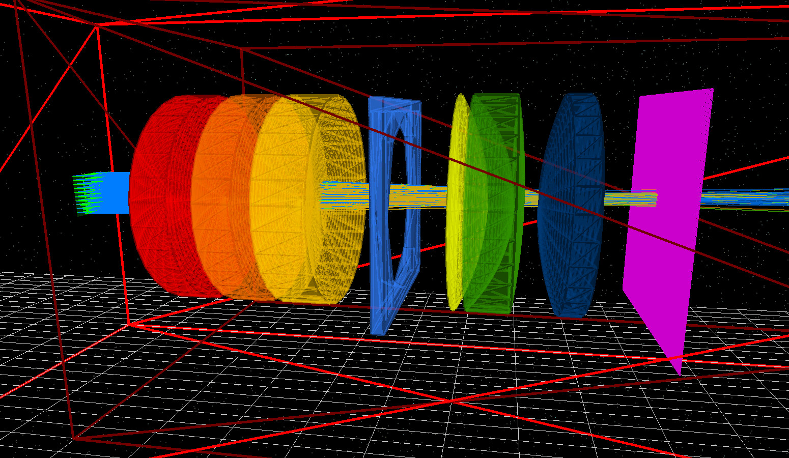
The ray-tracing solver propagates optical rays through a three-dimensional scene containing surfaces, bulk media, apertures, and detector planes. At each interface, the solver applies the appropriate geometric-optics update so that rays may be reflected, refracted, transmitted, or absorbed depending on the local material properties and geometry. In its most basic form, refraction is governed by Snell’s law,
\[ n_1 (\mathbf{k_i} \times \mathbf{n}) = n_2 (\mathbf{k_t} \times \mathbf{n}) \]
while interface reflection and transmission depend on the refractive indices and the local incidence geometry. In practical optical simulations, this means that lens curvature, spacing, aperture size, and wavelength-dependent refractive index all directly influence the final image and throughput of the system.
Unlike full-wave electromagnetic solvers, ray tracing is intended for problems where the optical wavelength is much smaller than the characteristic geometry and where light can be represented accurately by directed rays. This makes the method particularly efficient for multi-element lenses, macroscopic optical trains, microlens systems, and scattering or extraction problems in structured surfaces. It also makes the solver a natural partner to the rest of the OghmaNano optical toolchain, where geometric optics complements wave-based methods such as FDTD and transfer-matrix modelling.
Every ray-tracing simulation depends on three core ingredients: the source, the optical system, and the detector. In OghmaNano, the source is configured through the light-source editor, where the user can define beam shape, wavelength or spectral range, angular distribution, and emission characteristics. This makes it possible to model everything from simple collimated beams to more complex structured or multi-wavelength sources.
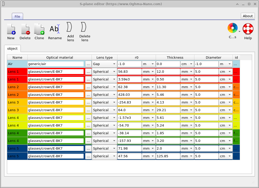
The optical system itself is constructed using three-dimensional geometry and, for lens-based systems, the S-plane editor. The S-plane provides a compact lens-design view in which radii, thicknesses, materials, diameters, and spacing can be edited directly while remaining tied to the underlying three-dimensional optical world. This is particularly useful for classical multi-element systems such as the Cooke triplet and for automated parameter scans over lens design space.
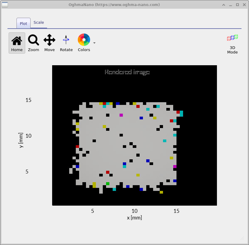
Detectors then measure the result of the optical system. These may record transmitted intensity, detector-plane images, efficiency versus wavelength, or other derived optical quantities depending on the simulation setup. Together, the source editor, S-plane editor, and detector tools turn the ray-tracing module into a practical environment for optical design, optical characterisation, and geometry-driven performance analysis.
One of the strengths of the OghmaNano ray-tracing environment is that it is not limited to single manual runs. Optical systems can be explored systematically using automated parameter scans and figures-of-merit analysis. This allows users to vary radii, thicknesses, spacing, aperture settings, or other geometric parameters across a batch of simulations and then compare the resulting optical performance quantitatively.
In practice, this makes the ray-tracing module useful not just for visualising rays, but for genuine optical design work. Spot size, detector efficiency, image quality, encircled-energy metrics, and related optical figures of merit can all be extracted and compared across parameter space. Users can therefore move from intuition-building visualisations to more systematic lens optimisation workflows without leaving the same environment.
This scan-and-optimise approach is especially valuable for multi-element systems where performance depends on several coupled design variables. It also makes the solver a practical platform for tolerance studies, design-space exploration, and rapid comparison of alternative optical layouts.
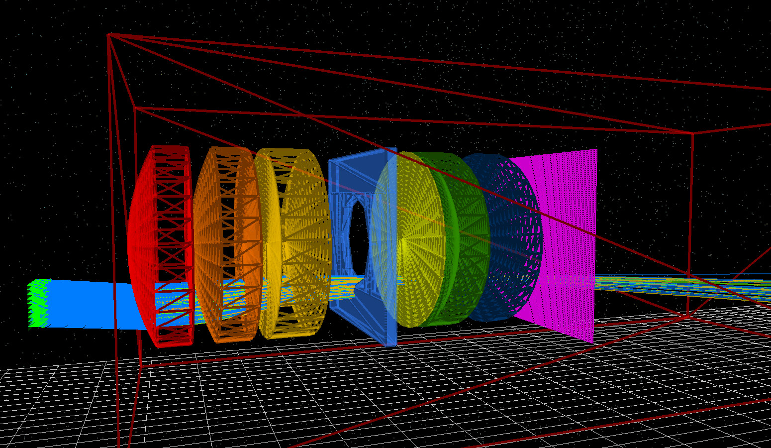
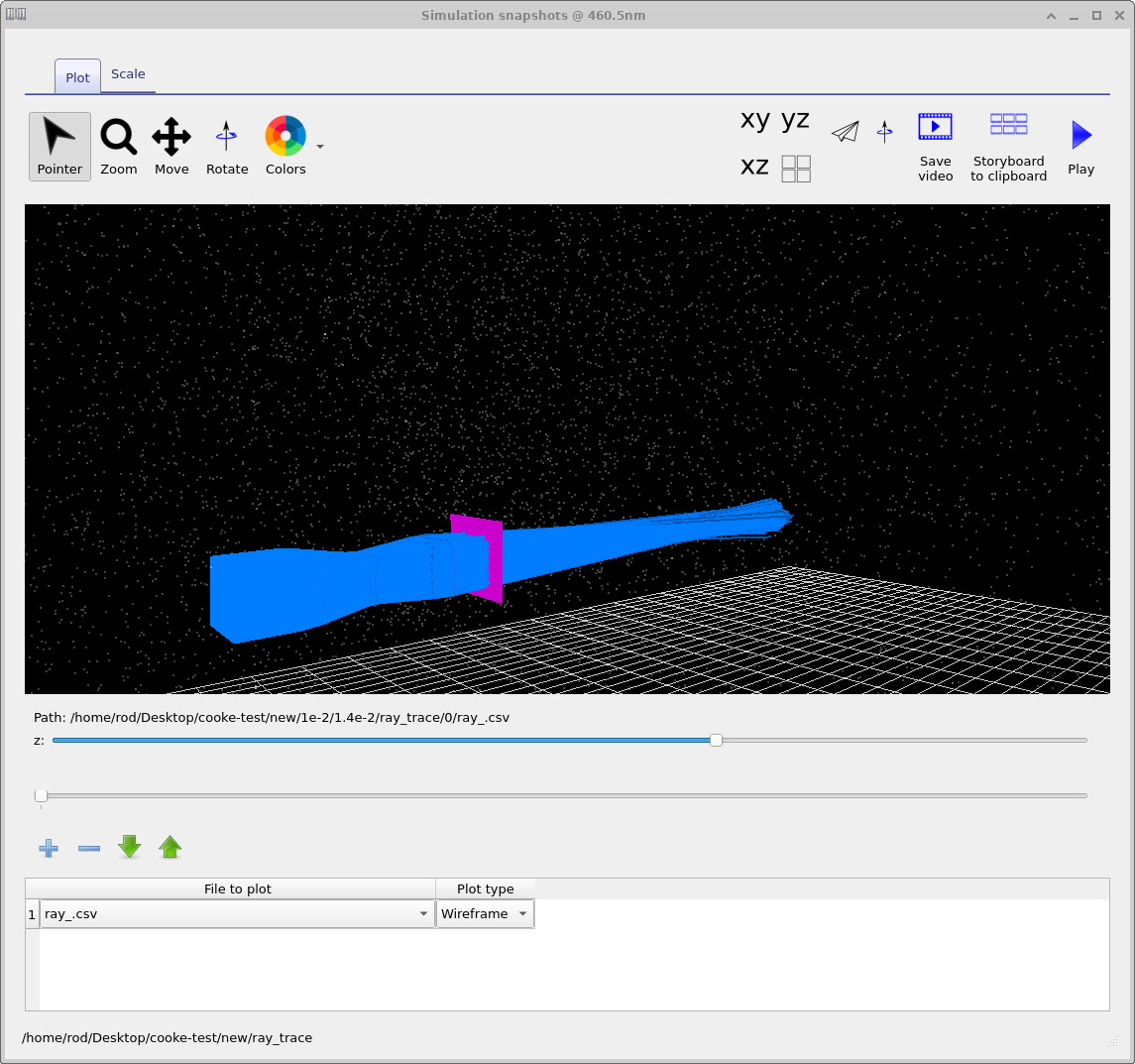
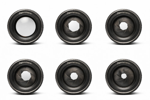
The ray-tracing solver can be used for a wide range of real optical problems. In imaging optics it can model multi-element lenses, apertures, focal planes, and detector images, as represented by Figure ??, Figure ??, and Figure ??. In these systems, the solver can be used to study aberrations, stop size, focusing behaviour, image formation, and wavelength-dependent throughput.
The same framework is also valuable for light interacting with films and structured surfaces, including rough-film reflection, escape from textured layers, and microlens-enhanced collection or filtering. Since the method works directly on three-dimensional geometry, it can also be used to study more complex optical assemblies where the full path of light through the structure matters.
Because OghmaNano supports wavelength sweeps, detector outputs, and automated scans, the solver is well suited both to quick exploratory simulations and to more systematic optical-design workflows. This makes it useful in contexts ranging from classical lens design to optoelectronic packaging and structured-surface optics.
OghmaNano includes a growing set of ray-tracing examples and step-by-step tutorials. These cover both introductory optical-system workflows and more advanced uses of parameter scans, figures of merit, rough surfaces, and microlens structures. They are intended to help users move quickly from a geometric model to a working optical simulation and then on to optimisation or analysis.
Useful starting points include the introduction to optical systems and ray tracing, the Cooke triplet lens tutorial, the 200 mm prime-lens example, the ray-tracing feature tour, the automated S-plane parameter scan tutorial, and the figures-of-merit workflow. For structured-surface optics, the rough-film reflection, light escape, and microlens demo show how the same ray-tracing engine can be used beyond classical lens systems.
Try a ray-tracing example.
Start with the introduction to optical systems and ray tracing, then move on to the Cooke triplet, prime-lens, or automated parameter scan tutorials.
To build your own systems, start with light sources, optical detectors, and the S-plane editor.