OghmaNano includes a simple equivalent circuit solver for modelling optoelectronic devices using compact SPICE-like resistor–capacitor–diode networks. This solver is intended for problems where a full drift–diffusion calculation would be unnecessarily detailed, too slow, or dependent on material parameters that are not known with confidence. Instead of solving the semiconductor transport equations throughout the device, the electrical response is represented by a small number of physically interpretable circuit elements.
This makes the solver particularly useful for rapid solar-cell modelling, shunt/series resistance analysis, compact JV fitting, transient response, impedance spectroscopy, EQE, and fast design optimisation. In the same workflow, OghmaNano can couple the circuit model to the transfer-matrix optical solver, so that a diode element receives a physically calculated photocurrent rather than an arbitrary fitted source term. In other words, the electrical model is simple and one-dimensional, while the optics can still retain full coherent thin-film interference.
For many practical device studies, this is exactly the right level of description. The equivalent circuit captures the dominant macroscopic behaviour — such as diode turn-on, series resistance losses, leakage through shunts, and geometric capacitance — while the optical engine determines how much light is actually absorbed in the chosen active layer. This makes the solver a natural bridge between fast compact modelling and physically meaningful optical coupling.
A full device-physics simulation can resolve carrier densities, electrostatic potential, recombination, traps, and transport in great detail, but this comes at a price: it requires many input parameters and a more expensive numerical solve. In contrast, the equivalent circuit solver reduces the problem to a handful of components with direct physical meaning. A solar cell, for example, is often well approximated by a diode in parallel with a shunt resistance and capacitance, plus a series resistance.
In this compact picture, the current can be written schematically as
\( I(V) = I_{0}\!\left[\exp\!\left(\frac{qV_{\mathrm{d}}}{nkT}\right)-1\right] - I_{\mathrm{ph}} \)
where \(I_{0}\) is the diode saturation current, \(n\) is the ideality factor, and \(I_{\mathrm{ph}}\) is the photocurrent. The voltage actually seen by the diode is modified by the surrounding circuit, particularly by the series and shunt elements. This is often enough to reproduce the key shape of a JV curve and to understand which loss channel is dominating the device.
When capacitive effects matter, the same circuit can also describe transient or frequency-domain behaviour using the usual relation
$$ I_{C} = C\,\frac{dV}{dt} $$
which makes the model suitable not only for steady-state JV sweeps, but also for CELIV, impedance spectroscopy, IMPS, and other modulated or transient measurements. That is one of the main strengths of the OghmaNano implementation: the circuit model is not a one-off toy solver, but a compact electrical engine embedded inside the broader experimental workflow of the software.
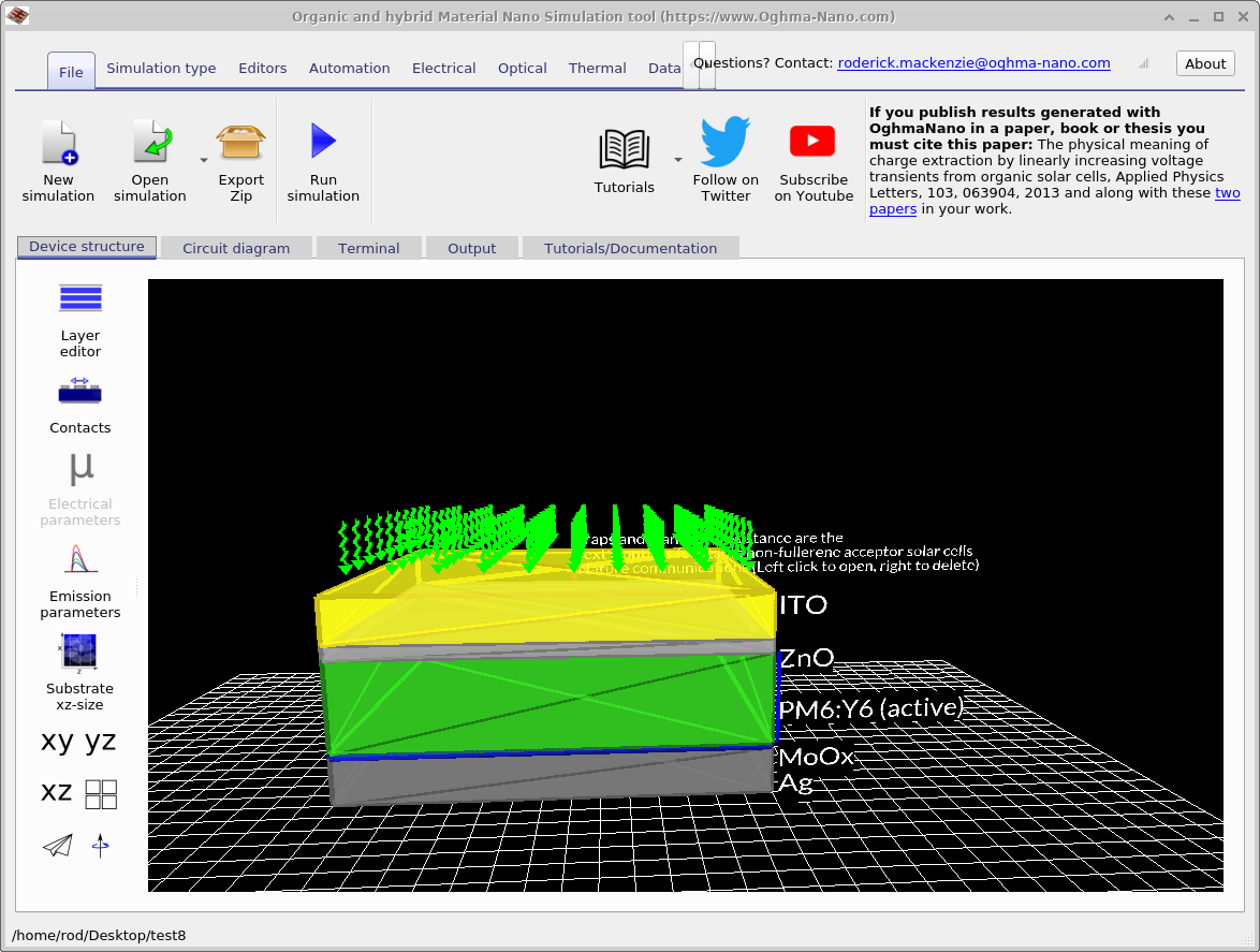
The most distinctive feature of the OghmaNano circuit solver is that it is not isolated from the optical physics. A diode can be linked to a specific layer in the device stack, and the photocurrent term can then be supplied by the transfer-matrix method (TMM). This means that the absorbed photon flux is calculated from the actual optical stack — including wavelength-dependent refractive index, thin-film interference, standing-wave effects, and position-dependent absorption — before being converted into a generation term for the circuit element.
This is extremely useful for solar cells, photodiodes, and other light-driven devices, because it allows you to explore how layer thickness, optical materials, and interference modify the current output without needing to run a full drift–diffusion model. In practice, this makes the equivalent circuit solver a powerful tool for fast architecture screening: you can test how a device responds electrically while still retaining a physically meaningful optical calculation.
Because the optical calculation is performed in the same software environment, it becomes easy to move between compact electrical modelling and more detailed optical design. You can, for example, modify the active-layer thickness in the stack, rerun the transfer-matrix calculation, and immediately observe the effect on the diode photocurrent and the final JV curve. This is one of the reasons the circuit solver is so effective for quick design optimisation of layered optoelectronic devices.
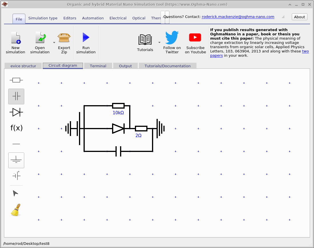
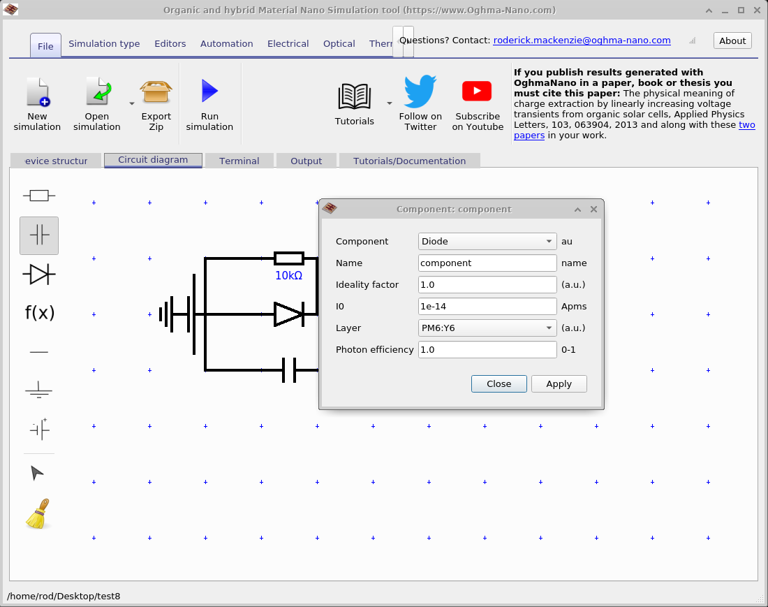
Circuit models are built using the Circuit Diagram tab in the main interface. The editor provides the standard building blocks needed for compact models: resistors, capacitors, diodes, non-linear elements, wires, ground, and sources. The example solar-cell circuit shown in Figure ?? contains the classic minimal photovoltaic network: a diode branch, a shunt branch, a series resistor, and a capacitor.
Clicking on a component opens an editor in which its parameters can be changed. For the diode, this includes the ideality factor, saturation current \(I_{0}\), the layer to which it is optically coupled, and the photon efficiency. This is shown in Figure ?? and Figure ??.
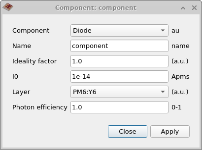
This component-level control is important because it lets you move smoothly from a purely fitted compact model to a semi-physical optoelectronic model. You can start with a simple ideal diode, then add realistic series resistance, shunt leakage, capacitive response, and finally optical generation from the transfer-matrix solver. That makes the editor useful for both teaching and research workflows.
A major advantage of the equivalent circuit engine is that it works inside the same simulation framework as the rest of OghmaNano. The applied voltage is defined in the same way as for a full device simulation, and the same experimental modes can be used. That means the compact model can be run in JV mode, EQE mode, Suns–VOC, Suns–JSC, CELIV, impedance spectroscopy, IMPS, capacitance–voltage, and other time- or frequency-domain modes.
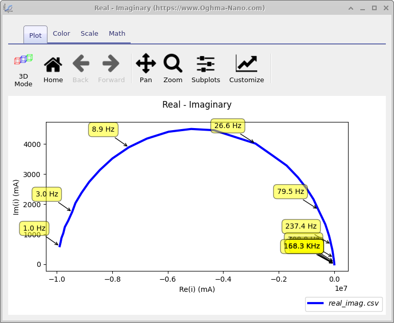
This is valuable because the same device can be explored from multiple perspectives without rebuilding the model in an external circuit package. The plot in Figure ?? shows a typical frequency-domain output, while the example below illustrates how the same circuit framework can also be used to calculate spectral outputs such as EQE. This makes the simple circuit solver much more than a basic JV-fitting tool. It can be used as a fast surrogate model for interpreting experiments, for testing how different equivalent-circuit parameters shape the measured response, and for rapidly screening designs before moving to more detailed device-physics simulations.
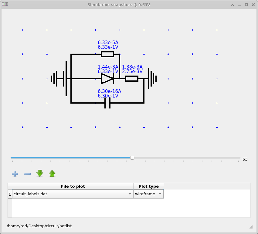
When the simulation is run from the main interface, the solver writes the usual output files to the Output tab. In addition, it can generate a netlist-style component output that records the current through and voltage across each element. This is especially useful for understanding which branch of the circuit is dominating the response at a given operating point.
The labelled circuit snapshot in Figure ?? shows this clearly: each component can be inspected as the slider moves through the sweep, allowing the user to see, for example, when the diode current becomes dominant, when the shunt path begins to matter, or how the capacitor contributes during a transient experiment.
This is one of the most instructive aspects of the solver. In a compact model, every element has a clear interpretation. Rather than inspecting a large field solve, you can directly ask: Is the fill factor being limited by series resistance? Is the low-voltage behaviour dominated by shunt leakage? Is the transient response capacitive? Is the photocurrent consistent with the optical absorption? The circuit outputs make those questions easy to answer.
The equivalent circuit solver is particularly well suited to:
It is also a good teaching tool. Because the model is simple and visual, it helps users build intuition for how diode quality, leakage paths, resistive losses, and optical generation combine to determine the final electrical response.
Because the solver is lightweight, it also works very well with OghmaNano’s scan and fitting tools. Circuit parameters are exposed in the same JSON-style parameter tree as the rest of the simulation, so they can be scanned, tuned, or fitted against experiment just like more detailed model parameters.
OghmaNano includes example compact models in the Simple Diode Models section of the simulation library. A good starting point is the Simple Equivalent Circuit tutorial, which introduces the circuit editor, explains the component parameters, and shows how the model can be coupled to the optical solver for a PM6:Y6-type solar cell.
Users interested in the optical side of the workflow should also look at the Transfer Matrix landing page and the thin-film optical filter tutorial, since the same coherent thin-film optics engine is responsible for generating the photocurrent term used by the diode. For more detailed electrical modelling beyond the compact approximation, see the Advanced Drift–Diffusion solver.
Try a simple circuit example.
Start with the Simple Equivalent Circuit tutorial to build and run a diode-based solar-cell model. Then explore alternative simulation modes such as JV, EQE, Suns–VOC, CELIV, and impedance spectroscopy using the same compact circuit.
To include physically meaningful photocurrent, combine the circuit model with the Transfer Matrix Method, which supplies absorption-driven generation directly to the diode element.