Fermi–Dirac vs Maxwell–Boltzmann statistics in semiconductors

Fermi–Dirac and Maxwell–Boltzmann statistics are used in semiconductor device modelling to relate carrier densities to the position of the quasi-Fermi levels. These statistics determine how electrons occupy available energy states within the density of states and therefore directly control carrier concentrations, electrostatics, recombination rates and transport behaviour.

This page explains how carrier densities in semiconductors are derived from the density of states and the Fermi–Dirac distribution, before deriving the Maxwell–Boltzmann approximation commonly used in drift–diffusion semiconductor device modelling. The differences between Fermi–Dirac and Maxwell–Boltzmann statistics, their physical meaning, computational cost and validity in degenerate and non-degenerate semiconductors are then discussed.

1. The density of states

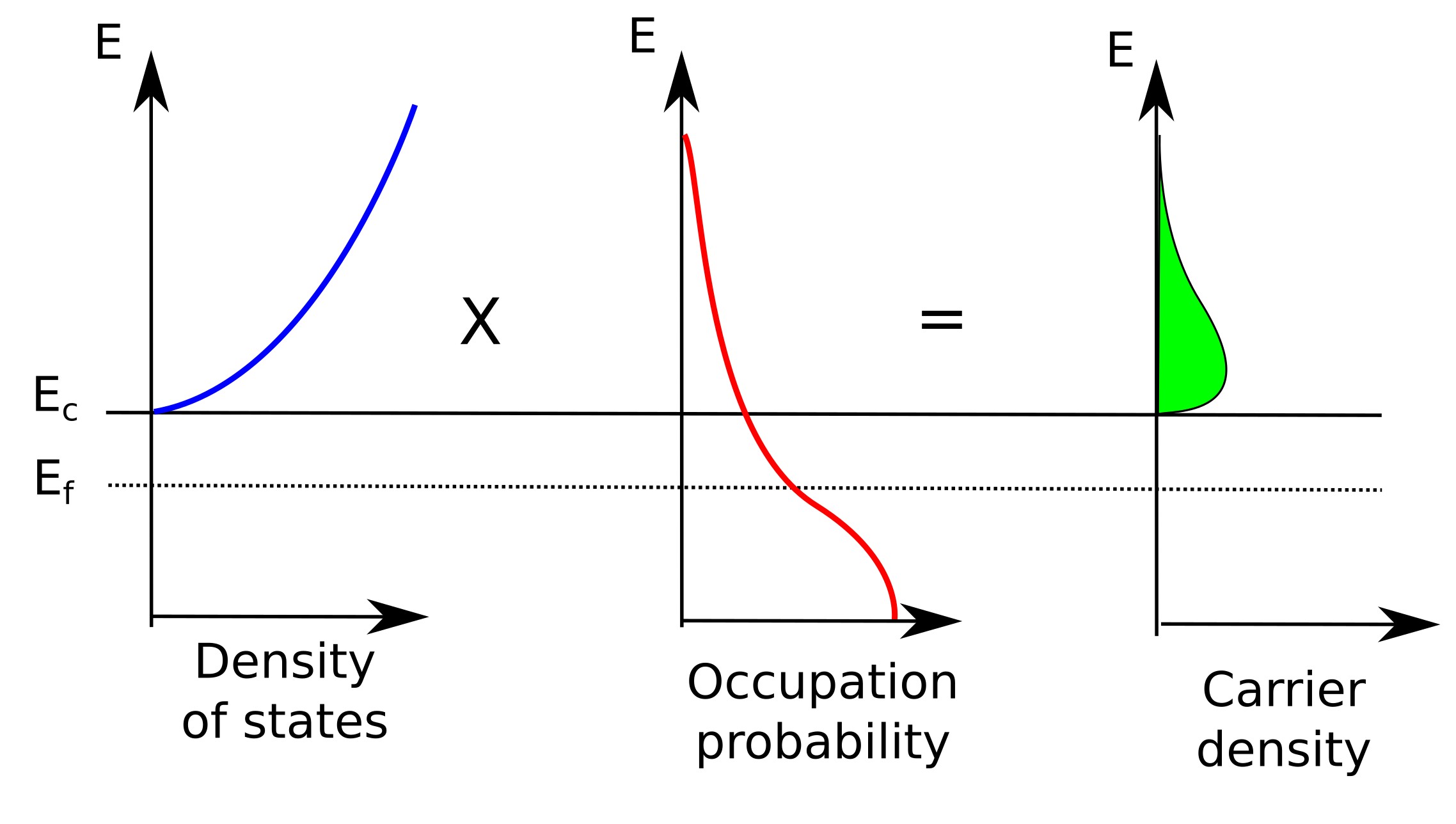
The density of states describes how many electronic states are available at each energy within the conduction band. Each state can hold one electron, or two electrons if spin is included. The distribution of available states is illustrated schematically in ??.

For a three-dimensional semiconductor with a parabolic conduction band, the density of states is given by

\[ g_{c}(E)=\frac{1}{2\pi^{2}} \left(\frac{2m_{n}^{*}}{\hbar^{2}}\right)^{3/2} \sqrt{E-E_{c}} \]

where \(g_{c}(E)\) is the density of states, \(m_{n}^{*}\) is the electron effective mass, \(\hbar\) is the reduced Planck constant and \(E_{c}\) is the conduction-band edge.

The density of states is zero below the conduction-band edge because no conduction-band states exist there. Above \(E_{c}\), the number of available states increases with energy.

2. Fermi–Dirac statistics

While the density of states describes how many electronic states are available at each energy, the Fermi–Dirac distribution describes the probability that each of these states is occupied by an electron. This distribution is illustrated schematically in ??.

\[ f(E)=\frac{1}{1+\exp\left(\frac{E-E_{F}}{k_{B}T}\right)} \]

Here, \(f(E)\) is the probability that a state of energy \(E\) is occupied by an electron, \(E_{F}\) is the Fermi level, \(k_{B}\) is Boltzmann's constant and \(T\) is temperature.

States well below the Fermi level are very likely to be occupied, while states far above the Fermi level are unlikely to contain electrons. Near the Fermi level, the occupation probability changes smoothly between filled and empty states.

3. Electron density in the conduction band using Fermi–Dirac statistics

The electron density in the conduction band is obtained by multiplying the density of states by the Fermi–Dirac occupation probability and integrating over energy, as illustrated in ??.

\[ \color{#008800}{n} \color{black}{=} \int_{E_{c}}^{\infty} \color{#0044ff}{g_{c}(E)} \color{#d00000}{f(E)} \color{black}{\,dE} \]

Substituting the conduction-band density of states and the Fermi–Dirac occupation function gives

4. Fermi–Dirac integral notation

The full carrier-density integral derived above does not generally have a simple analytical solution. Instead, it is commonly rewritten using the shorthand notation of the Fermi–Dirac integral.

This notation appears frequently in semiconductor physics because it provides a compact way of writing carrier statistics under degenerate conditions.

Here, \(F_{1/2}\) is the Fermi–Dirac integral of order one-half and \(N_c\) is the effective density of states of the conduction band.

\[ \color{#008800}{n} \color{black}{=} \int_{E_{c}}^{\infty} \color{#0044ff}{ \frac{1}{2\pi^{2}} \left(\frac{2m_{n}^{*}}{\hbar^{2}}\right)^{3/2} \sqrt{E-E_{c}} } \color{#d00000}{ \frac{1}{ 1+\exp\left(\frac{E-E_{F_n}}{k_{B}T}\right)} } \color{black}{\,dE} \]

Here, the blue term represents the number of available electronic states at each energy, while the red term represents the probability that these states are occupied by electrons.

3. Derivation of the Maxwell–Boltzmann approximation

The Maxwell–Boltzmann approximation is valid when the semiconductor is non-degenerate, meaning that the electron density is low enough that most electronic states in the conduction band remain empty. Under these conditions, the Fermi level lies several \(k_{B}T\) below the conduction-band edge, so that \(E-E_{F_n} \gg k_{B}T\) and the occupation probability satisfies \(f(E)\ll1\). Physically, this means electrons are sufficiently dilute that the Pauli exclusion principle does not strongly limit the occupation of states. In other words, electrons behave approximately like a classical gas because there are many more available states than electrons occupying them. This approximation is accurate for most conventional semiconductor devices operating at moderate carrier densities, including many silicon diodes, solar cells and organic semiconductor devices. However, it begins to break down at very high carrier densities, heavy doping levels or strong carrier accumulation, where a significant fraction of the available states become occupied. Under these conditions, \[ 1+\exp\left(\frac{E-E_{F_n}}{k_{B}T}\right) \approx \exp\left(\frac{E-E_{F_n}}{k_{B}T}\right) \] and the Fermi–Dirac distribution reduces to

\[ f(E)\approx \exp\left( -\frac{E-E_{F_n}}{k_{B}T} \right) \]

Substituting this into the carrier-density integral gives

\[ \color{#008800}{n} \color{black}{= \int_{E_{c}}^{\infty}} \color{#0044ff}{g_{c}(E)} \color{#d00000}{ \exp\left( -\frac{E-E_{F_n}}{k_{B}T} \right)} \color{black}{dE} \]

Evaluating the integral yields

\[ \color{#008800}{n} \color{black}{= N_{c} \exp\left( \frac{E_{F_n}-E_{c}}{k_{B}T} \right)} \qquad N_{c}=2 \left( \frac{2\pi m_{n}^{*}k_{B}T}{h^{2}} \right)^{3/2} \]

where \(N_c\) is the effective density of states of the conduction band. This is the standard Maxwell–Boltzmann carrier-density equation used in most drift–diffusion semiconductor device models.

4. When should I use Maxwell–Boltzmann statistics and when should I use Fermi–Dirac statistics?

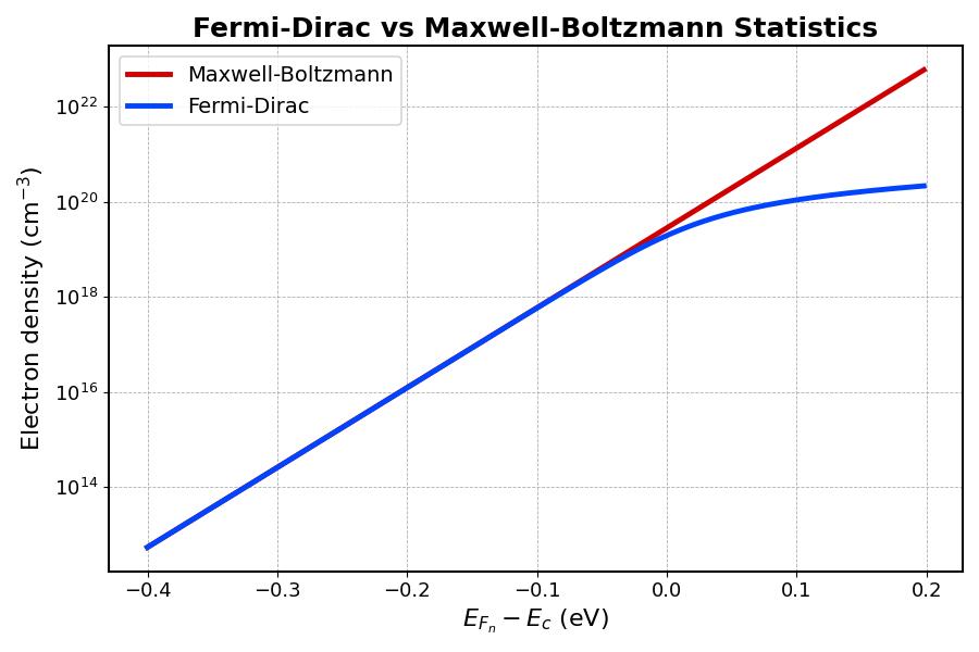
Maxwell–Boltzmann statistics should be used when the semiconductor is non-degenerate, meaning that the free carrier density is low enough that most states in the conduction and valence bands remain empty. Under these conditions, the quasi-Fermi levels remain several \(k_{B}T\) away from the band edges and state filling effects are negligible. This approximation is valid for most conventional semiconductor devices operating at moderate carrier densities, including many silicon pn junctions, OLED drift–diffusion simulations, organic photovoltaic devices and thin-film solar cells operating far from degeneracy.

In contrast, Fermi–Dirac statistics must be used for degenerate semiconductors, where the carrier density becomes sufficiently high that a significant fraction of the available electronic states become occupied. In these situations, the quasi-Fermi level approaches or enters a band and the Pauli exclusion principle strongly affects the carrier distribution. Examples where Fermi–Dirac statistics are often required include heavily doped semiconductors, quantum wells, highly injected LEDs, strong carrier accumulation layers and some inorganic laser structures.

In numerical semiconductor simulations, Maxwell–Boltzmann statistics are usually preferred whenever possible because the resulting carrier-density equations can be evaluated analytically and very efficiently. This makes the equations simpler, faster and numerically more stable. In contrast, Fermi–Dirac statistics are significantly slower to evaluate numerically because the carrier density must usually be obtained by explicitly evaluating the Fermi–Dirac integral. In practice, this often requires a numerical loop over energy or repeated evaluation of tabulated integrals, which introduces substantial computational overhead compared with the analytical Maxwell–Boltzmann approximation.

Therefore, when degenerate carrier populations do not need to be modelled, it is generally preferable to use Maxwell–Boltzmann statistics. However, when degenerate carrier populations are physically important, the full Fermi–Dirac statistics must be used to correctly capture state filling and carrier occupation effects. The discussion here concerns only the statistics of the free carrier populations in the conduction and valence bands. Very deep trap states generally require Fermi–Dirac occupation statistics regardless of whether the free carriers are degenerate, although this lies outside the scope of the present discussion.

5. Example scripts for plotting Fermi–Dirac and Maxwell–Boltzmann statistics

The difference between Maxwell–Boltzmann and Fermi–Dirac carrier statistics can be explored using the Python and MATLAB/Octave example scripts below. These scripts reproduce the behaviour illustrated in ?? and allow the effect of changing temperature, carrier density and quasi-Fermi level to be investigated interactively.

import math
import matplotlib.pyplot as plt

# Constants
k_B = 8.617333262e-5
T = 300.0
Nc = 2.8e19

# Generate energy axis
Ef_minus_Ec = []

x = -0.4

while x <= 0.2:
    Ef_minus_Ec.append(x)
    x += 0.002

# Maxwell-Boltzmann carrier density
n_mb = []

for eta in Ef_minus_Ec:
    n = Nc * math.exp(eta / (k_B * T))
    n_mb.append(n)

# Approximate Fermi-Dirac carrier density
n_fd = []

for eta in Ef_minus_Ec:

    arg = eta / (k_B * T)

    fd = Nc * math.log(1.0 + math.exp(arg))

    n_fd.append(fd)

# Plot
plt.figure(figsize=(7,5))

plt.semilogy(
    Ef_minus_Ec,
    n_mb,
    color='#d00000',
    linewidth=3,
    label='Maxwell-Boltzmann'
)

plt.semilogy(
    Ef_minus_Ec,
    n_fd,
    color='#0044ff',
    linewidth=3,
    label='Fermi-Dirac'
)

plt.xlabel(r'$E_{F_n}-E_c$ (eV)')
plt.ylabel(r'Electron density (cm$^{-3}$)')

plt.grid(True)
plt.legend()

plt.tight_layout()
plt.show()

k_B = 8.617333262e-5;
T = 300.0;
Nc = 2.8e19;

Ef_minus_Ec = -0.4:0.002:0.2;

n_mb = Nc .* exp(Ef_minus_Ec ./ (k_B*T));

arg = Ef_minus_Ec ./ (k_B*T);
n_fd = Nc .* log(1.0 + exp(arg));

semilogy(Ef_minus_Ec, n_mb, 'r', 'LineWidth', 3);
hold on;
semilogy(Ef_minus_Ec, n_fd, 'b', 'LineWidth', 3);

xlabel('E_F - E_c (eV)');
ylabel('Electron density');

legend('Maxwell-Boltzmann', 'Fermi-Dirac');

grid on;