

Perovskite/Silicon Tandem Solar Cell Simulation with Cross-Interface Recombination
1. Introduction: why combine perovskite and silicon?
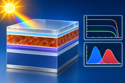
A perovskite/silicon tandem solar cell combines a wide-bandgap perovskite absorber with a lower-bandgap crystalline silicon absorber. The perovskite absorbs higher-energy photons, while light transmitted through the top cell can be absorbed by silicon. This can use the solar spectrum more efficiently than either subcell on its own.
This example is a monolithic, two-terminal (2T) tandem. The two subcells carry a common terminal current, while their photovoltages contribute to the overall voltage. Instead of explicitly resolving a thin interconnection semiconductor, the simulation uses a zero-thickness cross-interface recombination boundary between the perovskite and silicon regions.
The structure is a simplified teaching model rather than a fully calibrated industrial perovskite/silicon device. Its effective contact, recombination and band parameters are chosen to demonstrate how the electrical interconnection and optical generation work together.
💡 Tip: Modelling tandem solar cells. Tandem solar cells are more challenging to simulate than conventional single-junction devices because the top and bottom subcells must be electrically coupled through a recombination junction. The aim is to allow electrons from one subcell to recombine with holes from the other, connecting the two cells in series so that their voltages add together. There are two main ways to model this in OghmaNano:
1. Bulk recombination layer: Introduce a physical layer of finite thickness between the two subcells, with a high bimolecular recombination coefficient. This allows the recombination junction to be modelled explicitly, but very high recombination rates can introduce large terms into the Newton Jacobian matrix, sometimes leading to numerical instability. This approach is demonstrated in the perovskite/silicon tandem tutorial using a bulk recombination layer.
2. Cross-interface recombination: Instead of adding a separate layer, introduce a zero-thickness recombination interface between the two subcells. Conventional drift-diffusion transport across the interface is disabled, so electrons and holes cannot pass directly between the subcells. Instead, the cells are electrically connected through cross-interface electron-hole recombination. This avoids the need for an artificial recombination layer, although strong interface coupling can still introduce numerical convergence difficulties. This approach is demonstrated in the perovskite/silicon tandem tutorial using interface recombination and the organic tandem solar cell tutorial.
Both approaches aim to reproduce the electrical behaviour of a series-connected tandem solar cell. However, tandem simulations are generally more numerically demanding than single-junction simulations because the carrier populations, recombination rates and electrostatic potentials in the two subcells are strongly coupled. It is therefore important to monitor convergence and check that the total current is the same at both electrical contacts.
2. Opening the perovskite/silicon tandem example
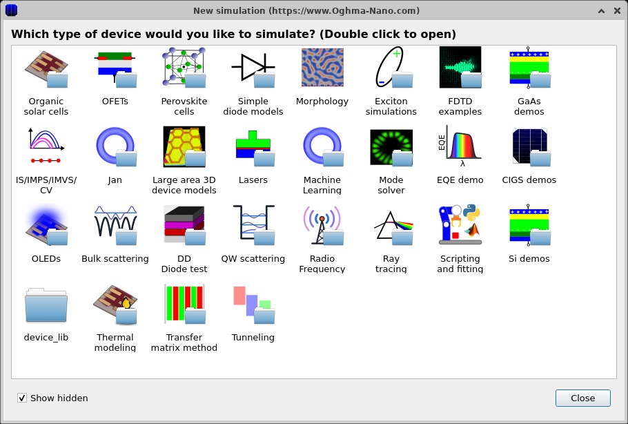
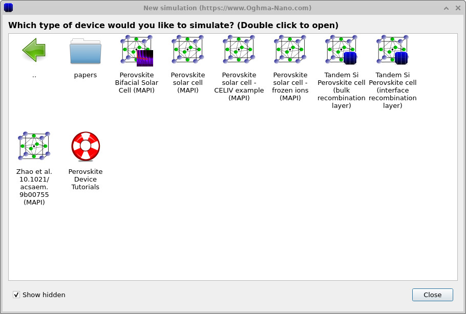
Start OghmaNano and select New simulation (??). In the perovskite examples, choose Tandem Si Perovskite cell (interface recombination layer), shown in ??. Do not confuse it with the separate bulk recombination layer example, which uses an electrically resolved interlayer.
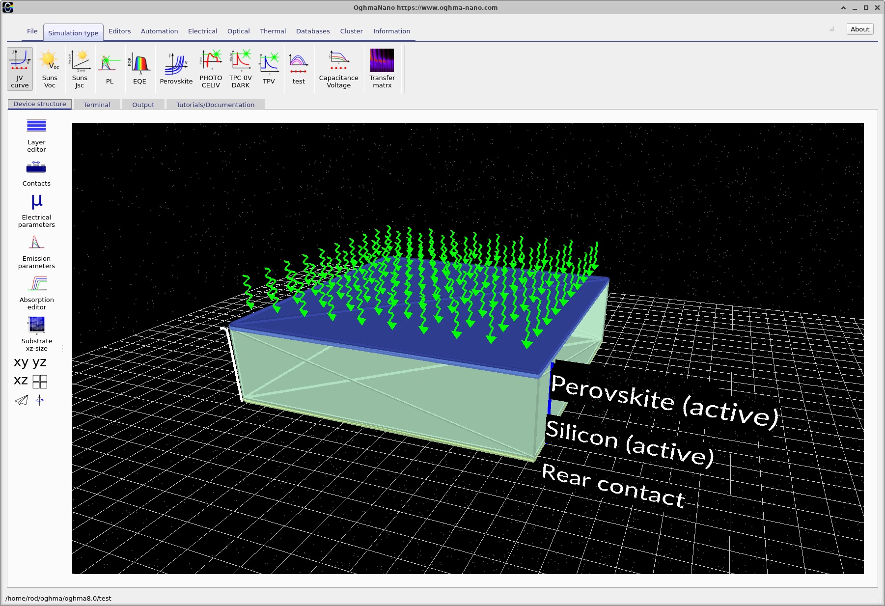
Save a copy before changing parameters. The Electrical ribbon gives access to the layer, contact and interface editors. The available simulation modes can be selected from the Simulation type ribbon (??).
💡 Tip: For best performance, save the simulation to a local drive such as C:\. Network, USB and synchronised cloud folders can be slow due to frequent file reads and writes.
3. Device structure and running the tandem simulation
The three-dimensional perovskite/silicon device structure is shown in ??. The example contains five layers, including a 500 nm perovskite top absorber and a 10 µm silicon bottom absorber. The two active semiconductor regions are connected by a cross-interface recombination boundary.
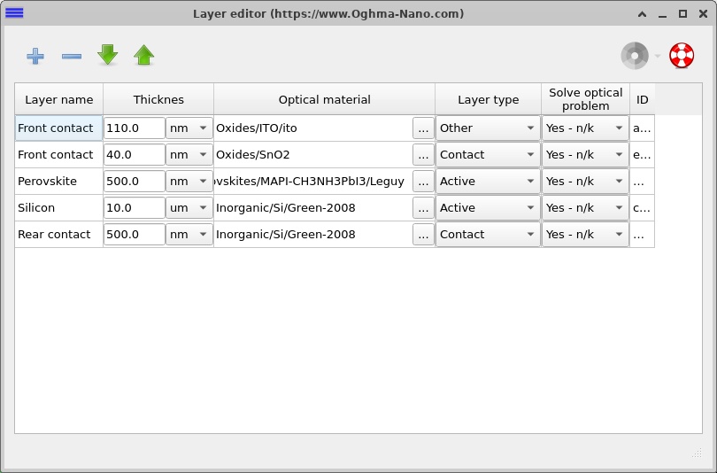
Click Layers in the Electrical ribbon to open the Layer editor, shown in ??. Layers marked Active are included in the drift-diffusion solution. Layers marked Other remain in the optical stack but are not separately solved as electrical semiconductor regions. Contact layers provide electrical boundary conditions and may also be represented in the optical stack. The contacts must be on the appropriate sides of the active stack.
| Layer (front to rear) | Thickness | Electrical role |
|---|---|---|
| Front contact (optical layer) | 110 nm | Other: included optically, not a resolved semiconductor region. |
| Front contact | 40 nm | Contact: defines the front electrical boundary condition. |
| Perovskite | 500 nm | Active: wide-gap top absorber. |
| Silicon | 10 µm | Active: lower-gap bottom absorber. |
| Rear contact | 500 nm | Contact: defines the rear electrical boundary condition. |
Run the simulation using the blue Run simulation button or F9. The terminal shows the progress of the Newton solver (??). This particular example uses a transfer-matrix generation profile for the electrical J-V calculation and sweeps applied voltage from −0.1 to 2.4 V.
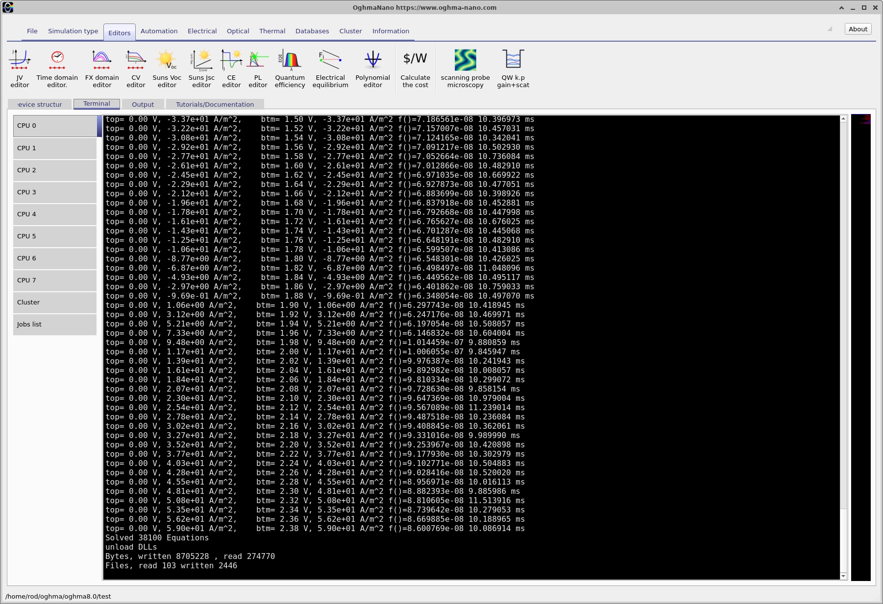
💡 Tip: Although the terminal output may look complicated, it is actually quite simple to read. Left and Right refer to the left and right electrical contacts. The voltage values show the voltage applied to each contact, while the current values show the current flowing through each contact. The value in the error brackets indicates how well the simulation has converged. An error exponent between approximately -6 and -11 indicates good convergence, whereas values between -2 and 1 suggest poor convergence. Finally, the time in milliseconds (ms) indicates how long that particular Newton iteration took to complete.
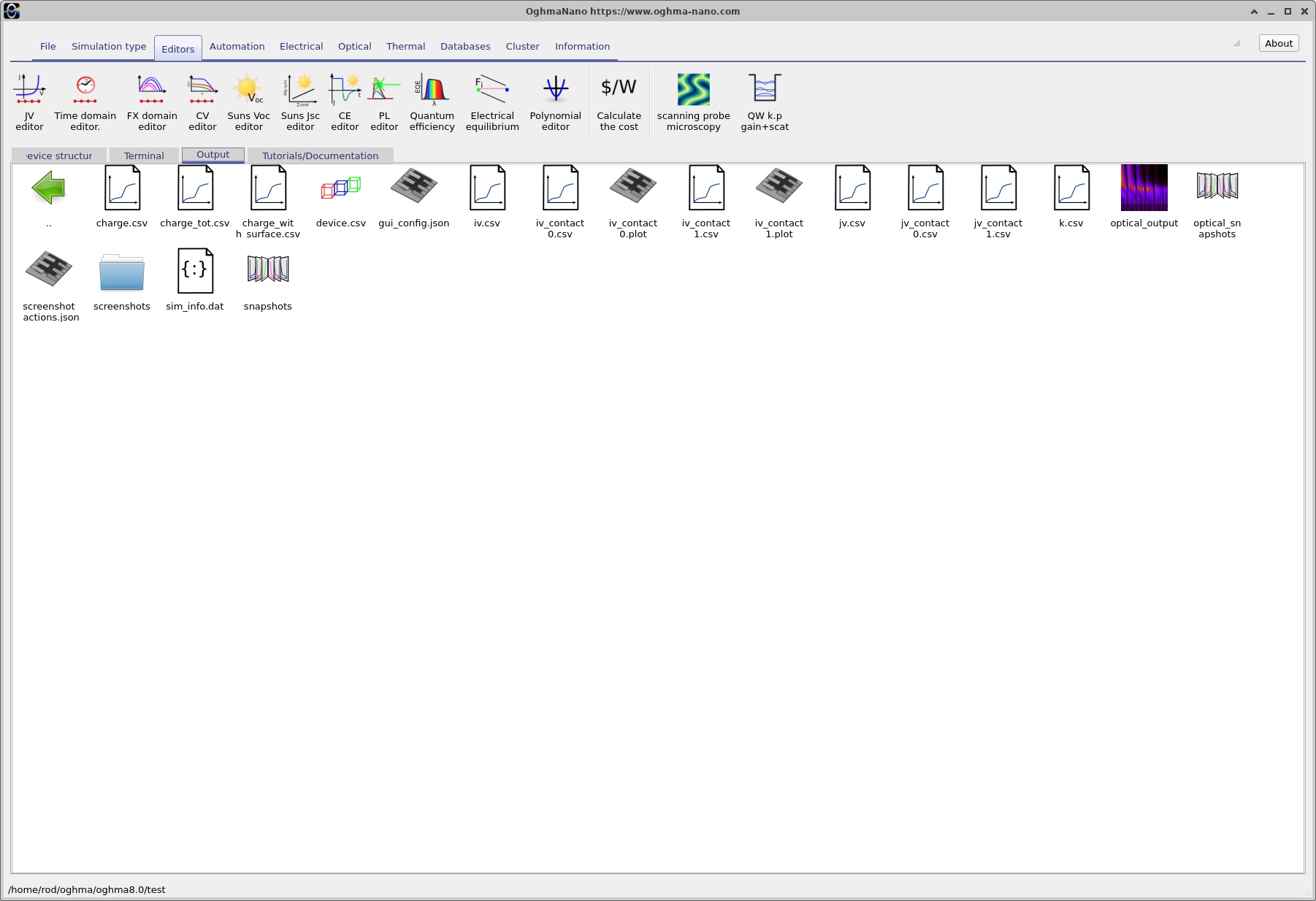
Once the calculation has finished, open the Output tab, shown in ??. This contains the files generated by the simulation, including the calculated J-V characteristic, internal carrier distributions and simulation information.
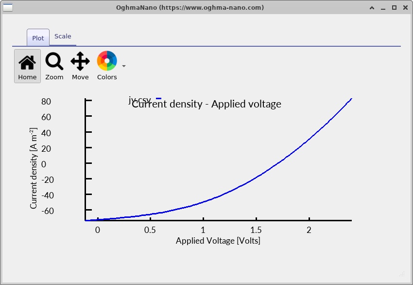
Double-click jv.csv to open the calculated current-voltage
characteristic
(??).
The two subcells are electrically connected in series, so they carry
the same current while their photovoltages contribute to the
total terminal voltage.
Double-click sim_info.dat to open the simulation information
(??).
This file contains information about the calculated device performance
and simulation settings. In the supplied example, the reported
VOC is approximately 1.71 V,
JSC approximately −72.4 A m−2
(−7.24 mA cm−2), fill factor about 0.402,
and power conversion efficiency approximately 4.97%.
These are demonstration results rather than experimentally validated performance figures.
jv.csv.
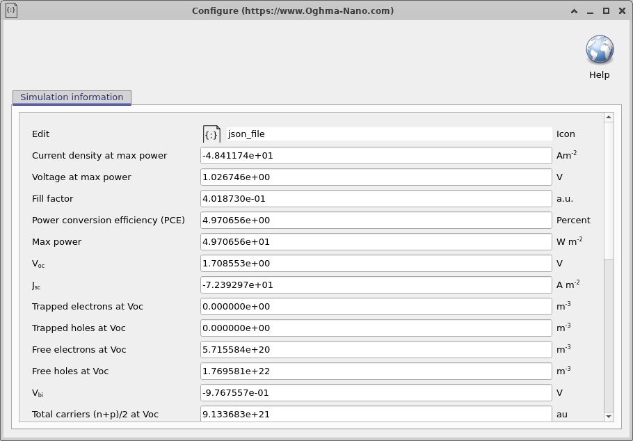
sim_info.dat.
4. Electrical parameters and bulk recombination
Click Electrical Parameters in the main OghmaNano window to inspect the carrier mobilities, effective densities of states, bandgaps and electron affinities. The two tabs for the perovskite and silicon regions are shown in ?? and ??.
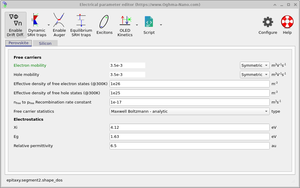
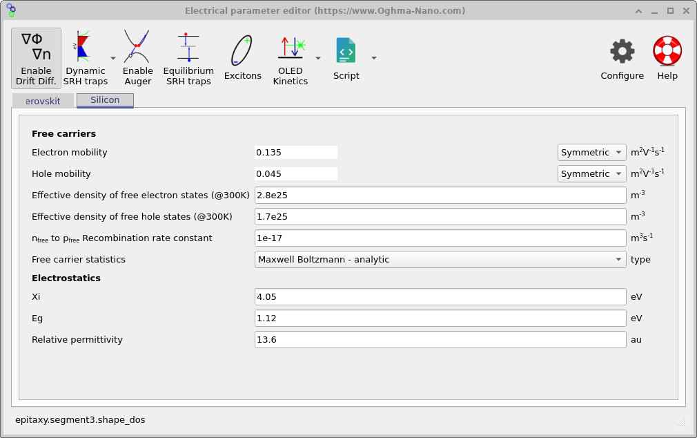
The simplified model uses the following parameters. The silicon region is represented by effective bulk transport parameters; the simulation does not resolve the full wafer processing sequence, textured interfaces or every selective contact layer.
| Parameter | Perovskite | Silicon |
|---|---|---|
| Thickness | 500 nm | 10 µm |
| Bandgap, Eg | 1.63 eV | 1.12 eV |
| Electron affinity, χ | 4.12 eV | 4.05 eV |
| Electron mobility, μn | 3.5 × 10⁻³ m² V−1 s−1 | 0.135 m² V−1 s−1 |
| Hole mobility, μp | 3.5 × 10⁻³ m² V−1 s−1 | 0.045 m² V−1 s−1 |
| Effective electron density of states, Nc | 1 × 1026 m−3 | 2.8 × 1025 m−3 |
| Effective hole density of states, Nv | 1 × 1025 m−3 | 1.7 × 1025 m−3 |
| Free-to-free recombination coefficient | 1 × 10⁻¹⁷ m³ s−1 | 1 × 10⁻¹⁷ m³ s−1 |
Both active regions use free-to-free (bimolecular) bulk recombination in this example. The associated coefficient is set to 10−17 m³ s−1 in each material. The single-level SRH option is not enabled in the supplied configuration, and the electrical model has no resolved multi-band SRH trap mesh.
\[ R_{\mathrm{bulk}}=B\left(np-n^{eq}p^{eq}\right). \]The bulk term describes recombination within each semiconductor. It is distinct from the cross-interface recombination that connects the two subcells electrically. In a more detailed or calibrated device model, the bulk loss mechanisms, doping, recombination coefficients and interface properties should be selected from experimental evidence.
5. The zero-thickness recombination junction
In a real tandem solar cell, the two photovoltaic junctions are connected through an interconnection or recombination layer. This region allows electrons arriving from one subcell to recombine with holes arriving from the other, providing an electrical connection between the two junctions. In practice, the interconnection may consist of several thin electron- and hole-selective transport layers together with a recombination-active material, such as a thin metal or conducting oxide.
One way to model this region is to insert an explicit thin semiconductor layer with a very high bimolecular recombination coefficient. Although this can reproduce the required recombination behaviour, combining extremely thin layers with very large recombination rates can make the numerical equations stiff and difficult to converge. A more efficient approach, particularly when the internal structure of the interconnection is not of interest, is to replace it with an infinitely thin recombination interface. This is the approach used in the present tandem simulation.
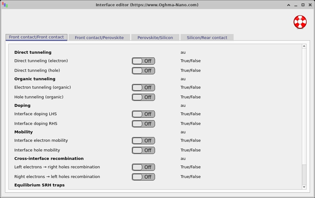
The interface is configured using the Interface editor, shown in ??. For further background on the underlying transport equations, see the semiconductor interface theory. Select the Perovskite/Silicon interface to inspect the recombination and transport parameters.
In this model, the electron and hole interface mobilities are both set to zero. This disables conventional electron and hole drift-diffusion transport across the boundary, effectively removing the ordinary transport terms connecting the neighbouring mesh points. Instead, the two subcells are electrically coupled through a cross-interface recombination mechanism, which allows an electron on one side of the interface to recombine directly with a hole on the other.
The recombination mechanism removes an electron on one side of the interface and a hole on the other. The two possible carrier pairings are described by
\[ R_{l2r}=K_{l2r}\left(n_Lp_R-n_L^{eq}p_R^{eq}\right), \] \[ R_{r2l}=K_{r2l}\left(n_Rp_L-n_R^{eq}p_L^{eq}\right). \]Here, \(L\) and \(R\) denote the mesh points immediately to the left and right of the interface, while the superscript \(eq\) denotes equilibrium carrier concentrations. The coefficients \(K_{l2r}\) and \(K_{r2l}\) have units of m4 s−1, giving recombination rates per unit area in m−2 s−1. The corresponding recombination current density is \(J_{\mathrm{rec}}=qR\). Subtracting the equilibrium carrier product ensures that the net recombination rate vanishes at thermal equilibrium.
In this example, the dominant channel couples electrons in silicon (right) to holes in perovskite (left). In the supplied configuration the coefficients are \(K_{r2l}=10^{-2}\,\mathrm{m^4\,s^{-1}}\) and \(K_{l2r}=10^{-25}\,\mathrm{m^4\,s^{-1}}\). The large difference between these values makes the recombination strongly directional, as required by the arrangement of the two photovoltaic junctions.
The purpose of the recombination interface is to provide an electrical connection between the subcells while allowing their individual photovoltages to add together. An efficient interconnection brings the relevant electron and hole quasi-Fermi levels close together at the centre of the device, minimising the voltage lost across the recombination junction.
Under Boltzmann statistics, the electron population on the right and the hole population on the left are related to their quasi-Fermi-level separation by
\[ n_Rp_L=n_R^{eq}p_L^{eq} \exp\left(\frac{E_{Fn,R}-E_{Fp,L}}{k_BT}\right). \]The recombination current can therefore be written as
\[ J_{\mathrm{rec}}= qK_{r2l}n_R^{eq}p_L^{eq} \left[ \exp\left(\frac{E_{Fn,R}-E_{Fp,L}}{k_BT}\right)-1 \right]. \]As the recombination coefficient increases, a smaller separation between \(E_{Fn,R}\) and \(E_{Fp,L}\) is needed to sustain the same current. In the strong-recombination limit, these two quasi-Fermi levels approach one another, creating an effective recombination contact between the subcells. This allows the photovoltage generated by each absorber to contribute to the overall tandem voltage, while reducing the voltage loss associated with the interconnection.
For two subcells connected electrically in series, the current density is common to both subcells; it is not the sum of their separate photocurrents. A photovoltaic J-V curve is commonly characterised by its short-circuit current density, open-circuit voltage and maximum-power point, provided the simulated bias range includes these operating points.
\[FF=\frac{|J_{mpp}V_{mpp}|}{|J_{SC}|V_{OC}},\qquad \eta=\frac{|J_{mpp}V_{mpp}|}{P_{in}}.\]Interpret the shape and sign of the displayed J-V trace using the simulation's current convention. The plotted example demonstrates the coupled electrical response; it should not be treated as an experimentally calibrated efficiency claim. Check the underlying CSV before reporting numerical performance figures.
💡 Tip: In this example, the electron and hole mobilities at the interface are set to zero. This disables conventional drift-diffusion transport across the interface, replacing it with a cross-interface recombination mechanism that electrically couples the two subcells. Both mechanisms can also be used together by assigning non-zero interface mobilities, although this may improve or worsen numerical stability depending on the device configuration.
The Right electrons → left holes recombination coefficient
controls the primary electrical coupling between the two subcells, allowing
electrons from the right subcell to recombine with holes from the left subcell.
Increasing this coefficient generally strengthens the coupling. However,
the recombination rate depends on the product of the electron and hole
concentrations, multiplied by the recombination coefficient. Consequently,
very large values, such as the 1e-2 used in the supplied example, can
introduce very large terms into the Newton Jacobian matrix and cause
numerical instability.
When adjusting the interface parameters, check that the left and right terminal currents agree in the simulation output. In a converged steady-state simulation, the total current must be the same at both contacts. A significant difference indicates a convergence or current-conservation problem.
The Left electrons → right holes recombination coefficient controls the opposite recombination pathway, allowing electrons from the left subcell to recombine with holes from the right subcell. In this device, it acts primarily as an additional recombination loss mechanism. Increasing it can substantially reduce the open-circuit voltage (VOC) and diminish the voltage advantage of the tandem structure. Conversely, reducing this coefficient suppresses unwanted recombination and can increase VOC.
6. Band structure and quasi-Fermi levels
To investigate how the two subcells operate electrically, open the
snapshots folder in the Output tab. This launches the
Snapshot Viewer, which allows the internal electrical
properties of the device to be examined at different applied voltages.
Click the + button and add the files
Ec.csv, Ev.csv, Fn.csv and
Fp.csv to display the conduction-band edge, valence-band
edge, electron quasi-Fermi level and hole quasi-Fermi level,
respectively. For further instructions, see the
Snapshot Viewer documentation.
The slider at the bottom of the window allows us to move through the voltage sweep. The four examples in ??–?? show the evolution of the band structure as the applied voltage increases across the simulated bias range. The plots cover a roughly 10 µm electrical stack, of which the upper 500 nm is perovskite and the remaining active region is silicon.
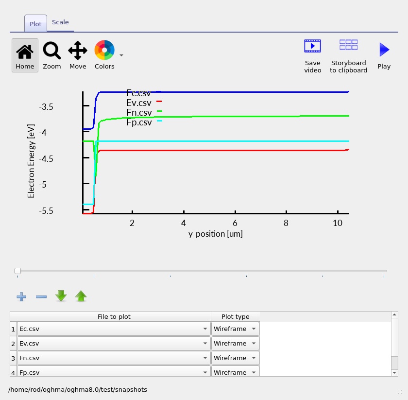
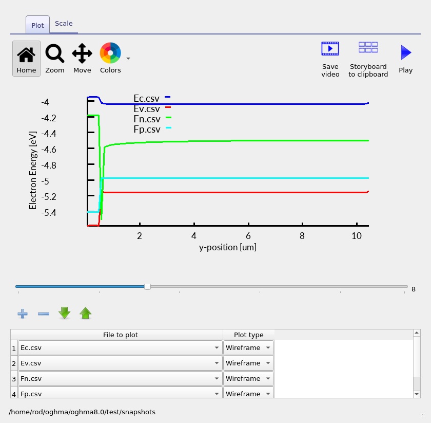
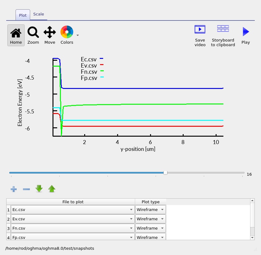
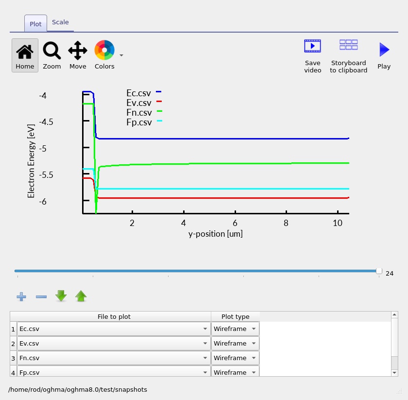
The blue and red curves represent the conduction and valence mobility edges, while the green and cyan curves represent the electron and hole quasi-Fermi levels. Under illumination, the separation between the electron and hole quasi-Fermi levels reflects the local nonequilibrium carrier populations and is closely related to the photovoltage generated by each subcell.
In a tandem solar cell, the two photovoltaic junctions are connected in series. Consequently, the voltage contributions from the two subcells add together. This can be seen particularly clearly in ??, which is close to the open-circuit condition. The quasi-Fermi-level splitting within each absorber contributes to the total terminal voltage, allowing the tandem to produce an open-circuit voltage of approximately 1.71 V in the supplied output, reflecting contributions from both semiconductor regions.
Another important feature is the sharp change in the quasi-Fermi levels at approximately 0.5 µm into the electrically active region, corresponding to the perovskite/silicon boundary. This is where the cross-interface recombination model connects the two subcells. The large recombination coefficient allows electrons on the right to recombine efficiently with holes on the left, tending to bring their respective quasi-Fermi levels towards the same energy.
This behaviour is particularly important for tandem operation. A strong recombination pathway allows the interface to carry current with only a small separation between the relevant quasi-Fermi levels, minimising the voltage lost at the interconnection. The quasi-Fermi-level profiles are also constrained by the local carrier currents and transport properties within each absorber. Consequently, the two subcells remain electrically connected while retaining their individual quasi-Fermi-level splitting and contributions to the overall tandem voltage.
7. Electron and hole current profiles
The electron and hole current densities provide another useful way to
understand how the two perovskite and silicon subcells are connected. Open the
snapshots folder from the Output tab and use the
+ button to add Jn.csv and
Jp.csv to the Snapshot Viewer. These files contain the
electron and hole current densities, respectively. The slider can
then be used to examine how the currents change as the applied
voltage increases. Further details on using this tool can be found
in the Snapshot Viewer documentation.
The four snapshots in ??–?? show the current distributions at four points through the applied-voltage sweep. The blue curve represents the electron current density, while the red curve represents the hole current density.
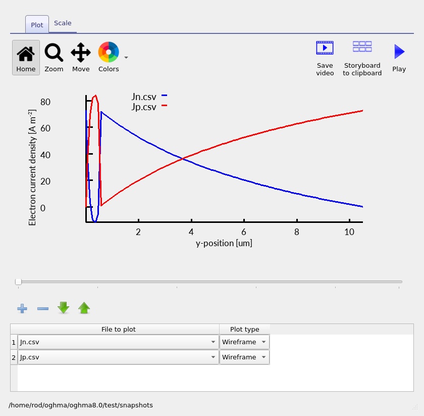
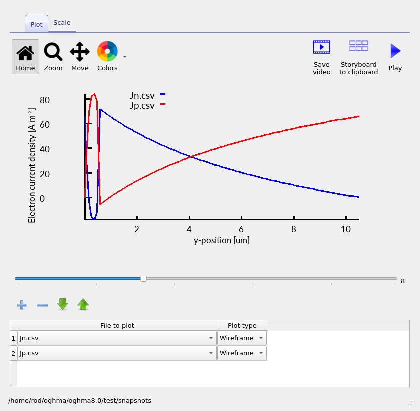
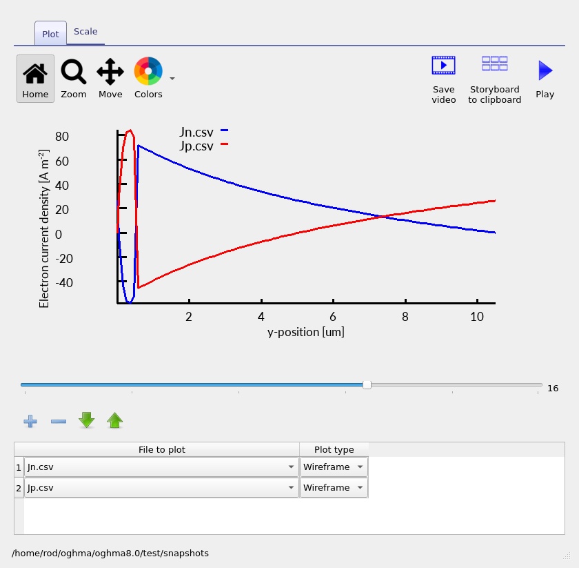
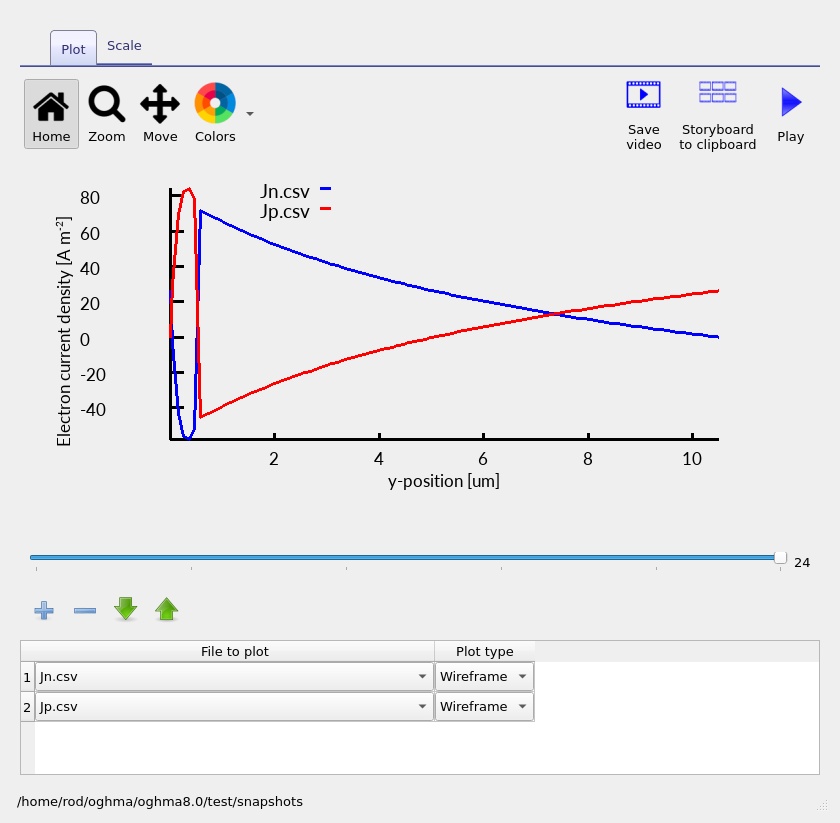
At low applied voltages in this example, the current is predominantly carried by electrons in perovskite on the left and holes in silicon on the right. At approximately 0.5 µm into the active stack, the boundary between the two absorbers, the electron current decreases sharply while the hole current increases. This is the characteristic behaviour of the recombination junction introduced in the previous section.
The cross-interface recombination mechanism removes an electron from one side of the interface and a hole from the other. Although the individual electron and hole currents can change abruptly at this boundary, their sum remains approximately constant:
\[ J_{\mathrm{total}}=J_n+J_p. \]This is an important result. In steady state, the total electrical current must be conserved through the complete tandem device, even though the relative contributions from electrons and holes change between the two subcells. The recombination interface provides the electrical connection without requiring carriers to drift or diffuse directly across the boundary.
Near the open-circuit voltage of approximately 1.71 V, the external current approaches zero. However, photogeneration and recombination continue within the device, so local electron and hole currents need not individually vanish. This helps explain why some snapshots show pronounced variations in the individual current components near the recombination interface, even though the overall terminal current is small.
Beyond the open-circuit voltage, the tandem is forward-biased and the terminal current changes sign. The magnitude of the injection current increases with bias. The same interfacial mechanism continues to operate: the dominant current changes between electron and hole transport at the centre of the device, while the total current remains continuous across the tandem.
The narrow peaks in the individual current components near the perovskite/silicon boundary (about 0.5 µm into the active stack) arise in the region where the strongly localised recombination boundary condition is applied. Their precise shape can depend on the spatial discretisation and numerical representation of the interface. The more important physical observation is that the two subcells remain electrically connected, with a conserved total current despite the abrupt redistribution between electron and hole currents.
8. Optical generation and transfer-matrix analysis
The wide-gap perovskite top cell absorbs a substantial fraction of the higher-energy solar photons, while the lower-gap silicon bottom cell can absorb longer-wavelength light transmitted through the perovskite. The transfer-matrix calculation accounts for absorption and interference throughout the optical stack.
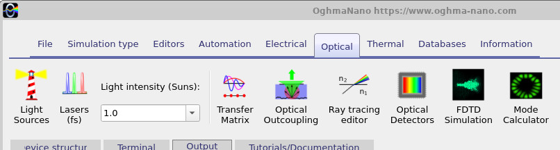
To inspect the optical behaviour, select the Optical ribbon in the main OghmaNano window, shown in ??, and click Transfer matrix. This opens the optical simulation editor. Click the blue Play button to run the optical calculation. The results can be explored using the tabs at the top of the optical simulation window, as shown in ??–??.
The transfer-matrix method calculates how light propagates through the multilayer device, accounting for reflections and interference at material interfaces. Each layer is described by its wavelength-dependent complex refractive index, \(\tilde{n}=n+ik\), where \(n\) determines the optical phase velocity and \(k\) describes absorption. Consequently, the optical intensity depends on both wavelength and position within the device.
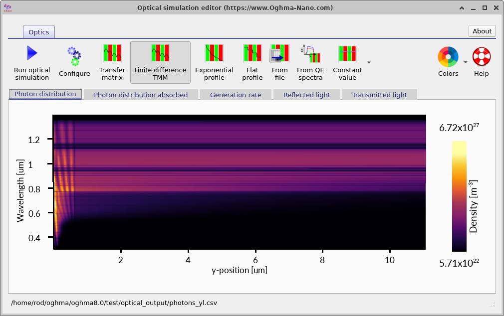
?? shows the photon density within the complete multilayer structure. The horizontal axis represents position through the device, while the vertical axis represents wavelength. The bright regions correspond to high photon densities, whereas dark regions indicate low photon densities. The variations arise from a combination of wavelength-dependent absorption and optical interference, which can produce standing-wave patterns within the thin-film stack.
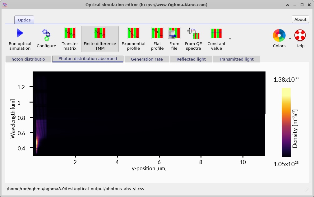
The absorbed photon distribution is shown in ??. Unlike photon density, this quantity describes where photons are actually absorbed. The perovskite and silicon regions have different spectral absorption windows. The perovskite preferentially absorbs higher-energy photons, while silicon can use longer wavelengths that pass through the upper cell. This complementary absorption behaviour is one of the principal motivations for combining these materials in a tandem solar cell.
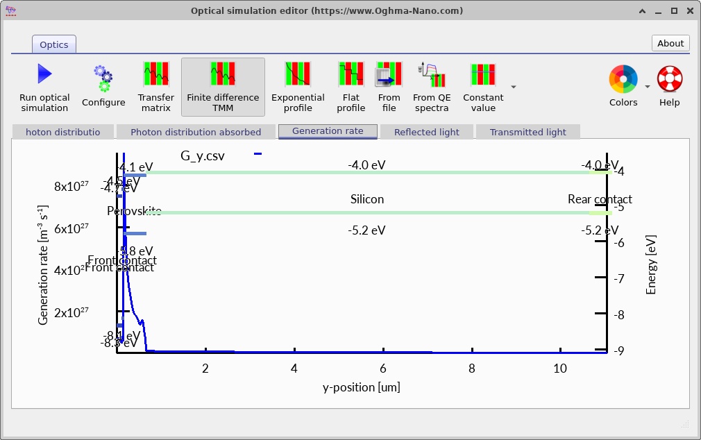
The spatial charge-carrier generation profile is shown in ??. The blue curve represents the calculated generation rate, while the horizontal energy levels indicate the positions of the different materials in the device. The generation profile extends across the thin perovskite top cell and the much thicker silicon bottom cell. Notice that the generation rate changes abruptly at the boundary between them, reflecting their different optical absorption properties.
The electrical generation rate is obtained by integrating the wavelength-dependent photon absorption over the incident spectrum:
\[ G(y)=\int \alpha(\lambda,y)\Phi(\lambda,y)\,d\lambda, \]where \(\alpha(\lambda,y)\) is the absorption coefficient and \(\Phi(\lambda,y)\) is the local spectral photon flux, defined per unit wavelength. The resulting generation rate has units of m−3 s−1 and provides the source term for photogenerated electrons and holes in the drift-diffusion equations. The conversion from absorbed photons to free carriers also depends on the photon-to-carrier generation efficiency used by the model.
An important consideration in tandem solar-cell design is current matching. Because the two subcells are electrically connected in series, they must carry the same terminal current. Increasing the absorption in the front subcell can reduce the number of photons reaching the rear subcell, potentially limiting the current of the complete device. The optimum absorber thicknesses therefore depend on the combined optical generation and electrical collection properties of both subcells, rather than simply maximising absorption in either material independently.
For a more detailed explanation of the optical method, see the Transfer Matrix Model tutorial and the transfer-matrix theory.
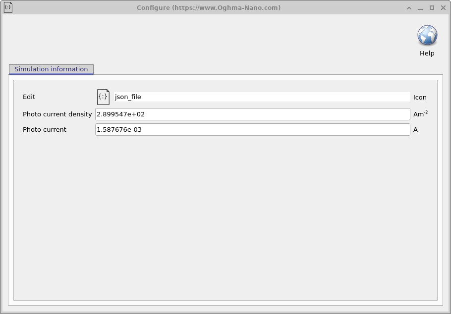
The optical output file siminfo.dat contains information about the optical simulation,
including the photocurrent and photocurrent density,
as shown in
??.
These values represent the maximum theoretical current that could be generated
if 100% of the photogenerated charge carriers were collected at the contacts,
with no recombination or charge-transport losses.
For a two-terminal tandem, the combined optical photocurrent is not itself the expected series-connected device current: the latter is constrained by current matching between the subcells.
These optical values therefore provide a photon-generation benchmark rather than a direct prediction of the tandem short-circuit current
(JSC).
9. Suns-Voc and Suns-Jsc simulations
OghmaNano provides several simulation modes for investigating how a device responds to different electrical and optical conditions. These can be selected from the Simulation type ribbon in the main window, shown in ??. Simply click the required simulation mode and press the blue Run simulation button or F9 to perform the calculation.
Two particularly useful simulations for solar cells are Suns-Voc and Suns-Jsc. These investigate how the open-circuit voltage and short-circuit current density change as the illumination intensity is varied. They provide complementary information about carrier generation, recombination and charge collection within the device.
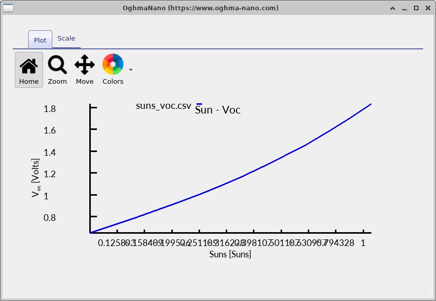
The Suns-Voc simulation calculates the open-circuit voltage at different illumination intensities. At open circuit, the external current is zero, so photogeneration must be balanced by recombination within the device. As illumination increases, the carrier concentrations generally increase, producing a larger separation between the electron and hole quasi-Fermi levels and therefore a higher open-circuit voltage.
For a simple illuminated diode, the relationship between open-circuit voltage and illumination intensity can be approximated by
\[ V_{OC} = \frac{n_{\mathrm{id}}k_BT}{q} \ln\left( \frac{J_{\mathrm{ph}}}{J_0}+1 \right), \]where \(n_{\mathrm{id}}\) is the diode ideality factor, \(k_B\) is Boltzmann's constant, \(T\) is temperature, \(q\) is the elementary charge, \(J_{\mathrm{ph}}\) is the photogenerated current density and \(J_0\) is the dark saturation current density. Since the photogenerated current is approximately proportional to illumination intensity, the open-circuit voltage generally increases logarithmically with the number of suns.
For a tandem solar cell, the measured voltage contains contributions from both photovoltaic subcells. To a first approximation,
\[ V_{OC,\mathrm{tandem}} \simeq V_{OC,1}+V_{OC,2}-V_{\mathrm{loss}}, \]where \(V_{\mathrm{loss}}\) represents any additional voltage loss associated with the interconnection. For an efficient recombination junction, this loss is small, allowing the photovoltages of the two subcells to add together.
The calculated Suns-Voc characteristic is shown in ??. The plot illustrates how the tandem voltage changes with light intensity. The variation is governed by the combined recombination and quasi-Fermi-level splitting of the two subcells; the exact numerical values should be read from the corresponding output file.
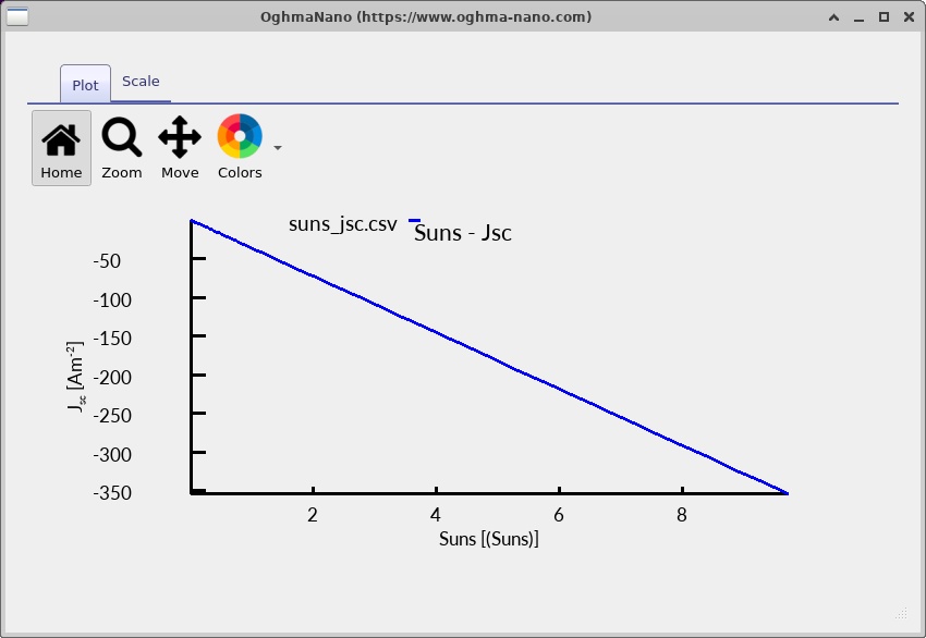
The Suns-Jsc simulation instead calculates the short-circuit current density as a function of illumination intensity. At short circuit, the applied terminal voltage is zero, and the measured current depends on the number of photogenerated carriers that can be collected.
If the collection efficiency remains approximately constant, the short-circuit current density is proportional to the incident photon flux. Consequently,
\[ |J_{SC}|\propto P_{\mathrm{sun}}, \]where \(P_{\mathrm{sun}}\) is the relative illumination intensity expressed in suns. More generally, the collected photocurrent depends on the spatial generation profile and the probability that photogenerated carriers reach the contacts:
\[ |J_{SC}| \simeq q\int G(y)\eta_{\mathrm{col}}(y)\,dy, \]where \(G(y)\) is the local photogeneration rate and \(\eta_{\mathrm{col}}(y)\) represents an effective position-dependent collection efficiency.
The Suns-Jsc output is shown in ??, and the corresponding characteristic is shown in ??. The calculated current density changes with illumination intensity. Inspect the numerical values in the plotted output to quantify the relationship. The negative sign in the plotted current reflects the photovoltaic current convention used by the solver.

suns_jsc.csv to examine the
calculated short-circuit current.
The two simulations highlight different aspects of tandem operation. Suns-Voc is particularly sensitive to the recombination processes that determine the achievable photovoltage, whereas Suns-Jsc provides information about photogeneration and charge collection. Because the two subcells are connected in series, they must carry the same terminal current, so the current generated by the complete tandem is constrained by the electrical and optical performance of both absorbers. Together, these calculations provide a useful way to investigate the behaviour of the tandem over a range of illumination conditions.
10. Suggested investigations
The central lesson is that optical stacking and electrical interconnection must be analysed together. The perovskite filters the spectrum reaching silicon, while the interface recombination mechanism provides the two-terminal series connection without an artificial electrically resolved intermediate semiconductor.