

Lua material scripting for semiconductor device simulation
OghmaNano supports Lua material scripting as an alternative to entering fixed material parameters individually through the graphical electrical parameter editor. For most simulations, fixed values entered through the GUI are sufficient; Lua scripting is intended for cases where electrical, optical, or thermal material properties need to be defined programmatically or vary with temperature, position (x, y, z), composition, or photon density. Parameters such as band gap, electron affinity, carrier mobility, recombination coefficients, and thermal conductivity can therefore be expressed as functions rather than single constants. This page explains how Lua material scripts are structured, how OghmaNano finds and selects them, how they are linked to materials and optical n/k datasets, and how scripted parameters are used within a simulation.
1. What is a Lua material script?
A Lua material script is a plain-text .lua file in which material properties are defined using small functions rather than fixed values. Each function returns the value of a particular material parameter, such as the band gap, electron affinity, carrier mobility, recombination coefficient, or thermal conductivity. These values can be constant, or they can vary as functions of temperature T and position (x, y, z). Functions can be enabled or disabled individually, allowing the script to override only the parameters you want while the remaining values continue to come from the standard simulation settings. A typical function looks like this:
function material.Eg(state)
	-- Band gap, units: eV
	local enabled = true
	local T = state.T
	local value = 1.42 - 4.5e-4*(T - 300.0)
	return value, enabled
end
Any .lua file in the OghmaNano Materials database is treated as a material script if the table declaration local material = {} appears within the first 1000 bytes of the file. This means a licence header or a block of explanatory comments can appear before the declaration, provided that the marker remains near the top of the file. You can view and edit a material's script directly from the Code editor tab in the Material editor
??.
A material script can define as much or as little as you like. It might define only the band gap and electron affinity, or a
full set of band-structure, transport, recombination, and thermal parameters. Functions you do not need can simply be left out,
or returned with enabled = false so that the model falls back to the value stored in the standard editors.
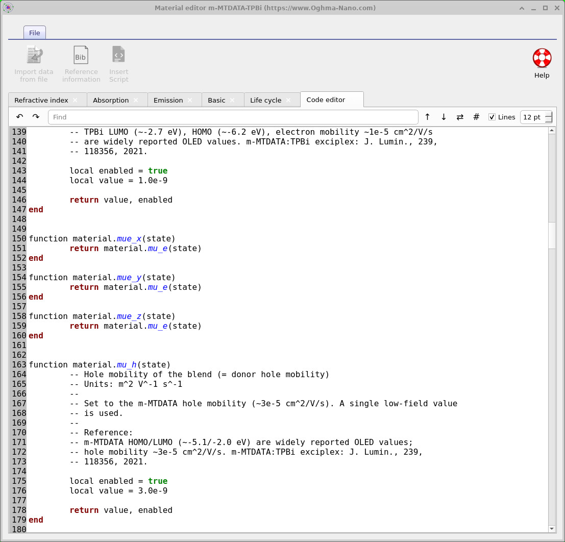
enabled flag.
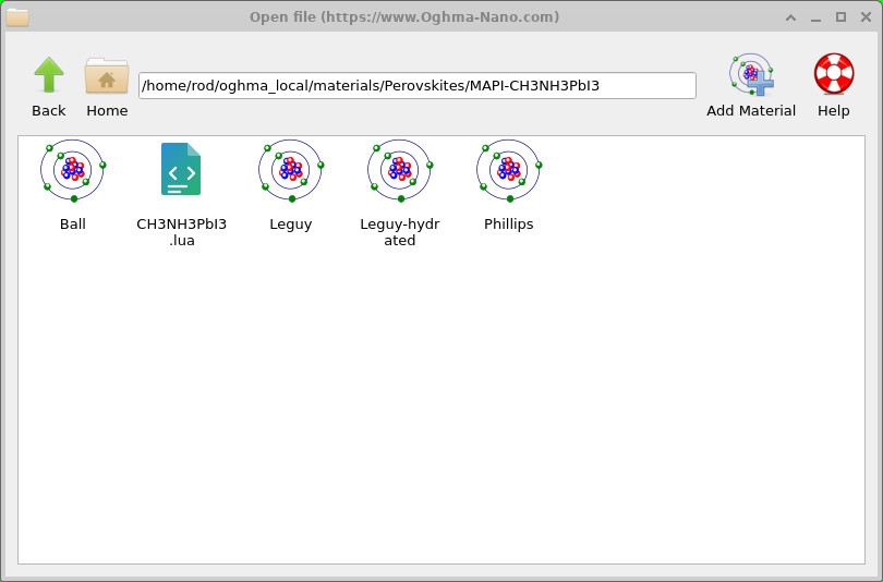
CH3NH3PbI3.lua). OghmaNano selects the most appropriate file for the simulation.
2. Where scripts live on disk
A material script can live in one of two places, and this determines how it appears in OghmaNano:
- Inside a material folder — for example inside the Gallium arsenide or MAPI-CH3NH3PbI3 folder. A script placed here belongs to that material and is displayed within the material when you open it, alongside its n/k data and other files.
-
Outside a material folder — a stand-alone
.luafile placed elsewhere in the database. In this case it is shown as a.luafile in its own right within the Materials database browser, rather than being attached to a single material.
Figure ?? shows a
script living inside a material folder. The MAPI-CH3NH3PbI3 perovskite folder contains several optical (n/k) datasets
— Ball, Leguy, Leguy-hydrated, and Phillips — represented by atom icons, together
with a single electrical script, CH3NH3PbI3.lua, represented by a code-file icon.
3. One electrical script, several optical datasets
It is common to have several sets of optical constants for one material but only one sensible set of electrical parameters. Different research groups measure n and k over different wavelength ranges, using different samples and different methods, so it is useful to keep each of those optical datasets separately and choose between them per simulation. The electrical parameters (band gap, affinity, mobilities, and so on), by contrast, are usually best kept as a single, consistent definition for the material. That is exactly the arrangement shown in ??: four n/k datasets, one electrical script.
When the material is used, OghmaNano tries to select the most appropriate file automatically. If a script is not present at the level of the specific material being simulated, the model will search backwards through the material folder structure to find a suitable script to use. This means you can attach one electrical script at a sensible level and have it apply to the datasets grouped beneath it, without having to duplicate the same electrical parameters into every optical variant.
Why separate the two? Optical data is often the thing that changes between measurements — a film measured to 800 nm by one group and to 1100 nm by another gives two legitimately different n/k datasets. The electrical behaviour of the material is not tied to the wavelength window of an optical measurement, so a single electrical script keeps the physics consistent no matter which optical dataset you pair it with.
4. Anatomy of a material script
The example below is a complete electrical material script for AlGaInAs — the lattice-matched InP-based quaternary used for telecom lasers and detectors. It is shown in full so you can see how a real, fully documented script is put together; each function is then broken out and explained in Section 5 below. Click to expand.
Full example material script — AlGaInAs.lua
-- See end of file for copyright, licensing and documentation links.

local material = {}

-- ---------------------------------------------------------------------------
-- NOTES ON AlGaInAs (read before using):
--
-- (Al_x Ga_{1-x})_{0.47} In_{0.53} As, LATTICE-MATCHED to InP (a = 5.869 A). The
-- workhorse quaternary for 1.3-1.55 um telecom lasers, modulators and
-- photodetectors. In is fixed at 0.53 for the InP match, so the single design
-- knob is the Al fraction x on the group-III sublattice.
--
-- DIRECT gap for all x (no crossover in the useful range): ~0.75 eV at x=0
-- (Ga0.47In0.53As, "InGaAs", ~1.65 um) rising to ~1.46 eV at x=1
-- (Al0.48In0.52As, ~0.85 um).
Show more
 -- Compared with the older InGaAsP telecom
-- quaternary, AlGaInAs offers a larger conduction-band offset (better electron
-- confinement), which is why it is favoured for high-temperature laser
-- operation - a device advantage, captured here only via Xi/Eg.
--
-- The lattice constant is FIXED by the InP match (independent of x). Eg is
-- computed from x; the remaining parameters are given at a representative
-- x = 0.30 (Eg ~ 0.92 eV, ~1.34 um) with InGaAs/AlInAs end points noted.
--
-- REFERENCES
--
-- [1]  I. Vurgaftman, J. R. Meyer, L. R. Ram-Mohan, J. Appl. Phys. 89, 5815
--      (2001). [constituent band parameters, bowing]
-- [2]  S. Adachi, "Properties of Semiconductor Alloys", Wiley (2009); and
--      S. Adachi, "Physical Properties of III-V Semiconductor Compounds"
--      (1992). [Eg(x), transport, dielectric, thermal]
-- [3]  O. Madelung, "Semiconductors: Data Handbook", Springer (2004).
-- ---------------------------------------------------------------------------

function material.name()
	local enabled = true

	return "AlGaInAs", enabled
end


function material.description()
	local enabled = true

	return "(AlxGa1-x)0.47In0.53As on InP, x = Al ~ 0.30 (direct gap)", enabled
end


function material.formula()
	local enabled = true

	return "AlGaInAs", enabled
end


function material.Eg(state)
	-- Units: eV
	-- Refs: [1],[2]
	--
	-- Direct gap, lattice-matched to InP, in Al fraction x. 300 K relation
	-- [2]:  Eg(x) = 0.76 + 0.49*x + 0.20*x^2
	-- (0.76 eV at x=0 -> 1.45 eV at x=1). Temperature handled by a
	-- Varshni-type shift about 300 K (alpha = 4.0e-4 eV/K, beta = 200 K).
	-- x = 0.30 -> ~0.925 eV (~1.34 um) at 300 K. Change al_fraction here
	-- and in the functions noted in the header.

	local enabled = true
	local al_fraction = 0.30
	local x = al_fraction
	local T = state.T
	local eg_300 = 0.76 + 0.49*x + 0.20*x*x
	local tshift = 4.0e-4*(90000.0/500.0 - T*T/(T + 200.0))
	local value = eg_300 + tshift

	return value, enabled
end


function material.Xi(state)
	-- Electron affinity
	-- Units: eV
	-- Refs: [2],[3]
	--
	-- ~4.45 eV at x = 0.30. Falls with Al (InGaAs ~4.6 -> AlInAs ~4.1 eV);
	-- the resulting large conduction-band offset to InP / across the alloy
	-- is the key confinement advantage over InGaAsP.

	local enabled = true
	local value = 4.45

	return value, enabled
end


function material.Nc(state)
	-- Effective conduction-band density of states
	-- Units: m^-3
	-- Refs: [2],[3]
	--
	-- ~4e23 m^-3 at 300 K for x = 0.30 (small direct-valley mass, m_e* ~
	-- 0.05-0.07 m0). Endpoints: InGaAs ~2.1e23, AlInAs ~5.4e23 m^-3.

	local enabled = true
	local T = state.T
	local value = 4.0e23*(T/300.0)^1.5

	return value, enabled
end


function material.Nv(state)
	-- Effective valence-band density of states
	-- Units: m^-3
	-- Refs: [2],[3]
	--
	-- ~8e24 m^-3 at 300 K for x = 0.30 (InGaAs ~7.7e24, AlInAs ~9e24 m^-3).

	local enabled = true
	local T = state.T
	local value = 8.0e24*(T/300.0)^1.5

	return value, enabled
end


function material.mu_e(state)
	-- Low-field electron mobility
	-- Units: m^2 V^-1 s^-1
	-- Refs: [2]
	--
	-- ~0.3 m^2/V/s (3000 cm^2/V/s) at x = 0.30 - high (small mass) but
	-- alloy-scattering-reduced from InGaAs (~10000-13000 cm^2/V/s) toward
	-- AlInAs (~1000-4000 cm^2/V/s). (300/T)^1.5 approximate.

	local enabled = true
	local T = state.T
	local value = 0.30*(300.0/T)^1.5

	return value, enabled
end

function material.mue_x(state)
	return material.mu_e(state)
end

function material.mue_y(state)
	return material.mu_e(state)
end

function material.mue_z(state)
	return material.mu_e(state)
end


function material.mu_h(state)
	-- Low-field hole mobility
	-- Units: m^2 V^-1 s^-1
	-- Refs: [2]
	--
	-- ~0.02 m^2/V/s (200 cm^2/V/s) at x = 0.30 (InGaAs ~300, AlInAs ~100
	-- cm^2/V/s). (300/T)^1.5 approximate.

	local enabled = true
	local T = state.T
	local value = 0.02*(300.0/T)^1.5

	return value, enabled
end

function material.muh_x(state)
	return material.mu_h(state)
end

function material.muh_y(state)
	return material.mu_h(state)
end

function material.muh_z(state)
	return material.mu_h(state)
end


function material.epsilonr(state)
	-- Relative static permittivity
	-- Dimensionless
	-- Refs: [2],[3]
	--
	-- ~13.4 at x = 0.30 (InGaAs ~13.9 -> AlInAs ~12.5).

	local enabled = true
	local value = 13.4

	return value, enabled
end


function material.free_to_free_recombination(state)
	-- Radiative recombination coefficient
	-- Units: m^3 s^-1
	-- Refs: representative (see note)
	--
	-- Direct-gap value ~1e-10 cm^3/s = 1e-16 m^3/s. Representative; refine
	-- against measured lifetimes.

	local enabled = true
	local value = 1.0e-16

	return value, enabled
end


function material.auger_Cn(state)
	-- Electron Auger recombination coefficient
	-- Units: m^6 s^-1
	-- Refs: representative (see note)
	--
	-- ~2e-28 cm^6/s = 2e-40 m^6/s at the InGaAs-rich (narrow-gap) end.
	-- Auger is a major loss mechanism in 1.55 um AlGaInAs/InGaAsP lasers
	-- and grows sharply as x decreases (gap narrows) - scale accordingly.

	local enabled = true
	local value = 2.0e-40

	return value, enabled
end


function material.auger_Cp(state)
	-- Hole Auger recombination coefficient
	-- Units: m^6 s^-1
	-- Refs: representative (see note)
	--
	-- As auger_Cn: representative 2e-28 cm^6/s = 2e-40 m^6/s.

	local enabled = true
	local value = 2.0e-40

	return value, enabled
end


function material.ss_srh_trap_energy(state)
	-- SRH trap energy relative to the middle of the band gap.
	-- Units: eV
	--
	-- Positive values are above mid-gap (towards the conduction band).
	-- Negative values are below mid-gap (towards the valence band).
	--
	-- Defect-dependent. Lattice-matched InP-based material can be very high
	-- quality; set level and density from your own data. Mid-gap default.

	local enabled = true
	local value = 0.0

	return value, enabled
end


function material.ss_srh_Nt(state)
	-- SRH trap density
	-- Units: m^-3
	--
	-- Defect-dependent placeholder; set from the intended material
	-- quality.

	local enabled = true
	local value = 1.0e21

	return value, enabled
end


function material.ss_srh_sigma_n(state)
	-- Electron capture cross section
	-- Units: m^2
	--
	-- Defect-dependent placeholder; set from measurement.

	local enabled = true
	local value = 1.0e-19

	return value, enabled
end


function material.ss_srh_sigma_p(state)
	-- Hole capture cross section
	-- Units: m^2
	--
	-- Defect-dependent placeholder; set from measurement.

	local enabled = true
	local value = 1.0e-19

	return value, enabled
end


function material.thermal_kl(state)
	-- Thermal conductivity
	-- Units: W m^-1 K^-1
	-- Refs: [2]
	--
	-- ~4.5 W/m/K at x = 0.30 - LOW, from strong mass-disorder phonon
	-- scattering in this quaternary (well below InP's ~68 or InAs's ~27
	-- W/m/K). Weakly dependent in the alloy regime; (300/T)^0.4 approximate.
	-- This low kappa contributes to self-heating in InP-based lasers.

	local enabled = true
	local T = state.T
	local value = 4.5*(300.0/T)^0.4

	return value, enabled
end


function material.heat_capacity(state)
	-- Specific heat capacity
	-- Units: J kg^-1 K^-1
	-- Refs: [3]
	--
	-- ~320 J/kg/K near 300 K (interpolated across the constituents).

	local enabled = true
	local value = 320.0

	return value, enabled
end


function material.density(state)
	-- Mass density
	-- Units: kg m^-3
	-- Refs: [3]
	--
	-- ~5300 kg/m^3 at x = 0.30 (InGaAs ~5500 -> AlInAs ~4650 kg/m^3).

	local enabled = true
	local value = 5300.0

	return value, enabled
end


function material.lattice_constant(state)
	-- Cubic lattice constant
	-- Units: m
	-- Refs: [1],[3]
	--
	-- FIXED at the InP match, a = 5.8697 A, INDEPENDENT of x (Al substitutes
	-- for Ga at constant lattice constant along the InP-matched line).
	-- Linear thermal expansion ~4.6e-6 /K (InP-like).

	local enabled = true
	local T = state.T
	local a300 = 5.8697e-10
	local expansion = 4.6e-6
	local value = a300*(1.0 + expansion*(T - 300.0))

	return value, enabled
end


function material.thermal_tau_e(state)
	-- Electron energy relaxation time towards the lattice temperature
	-- Units: s
	--
	-- Value basis: III-V family estimate
	-- Confidence: Medium
	--
	-- Reference:
	-- https://www.mdpi.com/2673-3978/3/2/16
	--
	-- Comments:
	-- Representative III-V carrier-to-lattice relaxation time. GaAs-like values
	-- are typically sub-ps to ps and field dependent.

	local enabled = true
	local value = 5.000000e-13

	return value, enabled
end


function material.thermal_tau_h(state)
	-- Hole energy relaxation time towards the lattice temperature
	-- Units: s
	--
	-- Value basis: III-V family estimate
	-- Confidence: Medium
	--
	-- Reference:
	-- https://www.mdpi.com/2673-3978/3/2/16
	--
	-- Comments:
	-- Representative III-V carrier-to-lattice relaxation time. GaAs-like values
	-- are typically sub-ps to ps and field dependent.

	local enabled = true
	local value = 5.000000e-13

	return value, enabled
end


function material.print()
	local state = {
		T = 300.0,
		x = 0.0,
		y = 0.0,
		z = 0.0,
		photon_density = 0.0,
	}

	print(string.format("Material:               %s", material.name()))
	print(string.format("Description:            %s", material.description()))
	print(string.format("Formula:                %s", material.formula()))
	print(string.format("Temperature:            %.2f K", state.T))
	print(string.format("Position:               %.6e, %.6e, %.6e m", state.x, state.y, state.z))
	print(string.format("Photon density:         %.6e m^-3", state.photon_density))

	print(string.format("Band gap:               %.6f eV", material.Eg(state)))
	print(string.format("Electron affinity:      %.6f eV", material.Xi(state)))
	print(string.format("Electron mobility:      %.6e m^2/V/s", material.mu_e(state)))
	print(string.format("Hole mobility:          %.6e m^2/V/s", material.mu_h(state)))
	print(string.format("Nc:                     %.6e m^-3", material.Nc(state)))
	print(string.format("Nv:                     %.6e m^-3", material.Nv(state)))
	print(string.format("Relative permittivity:  %.6f", material.epsilonr(state)))

	print(string.format("Radiative coeff.:       %.6e m^3/s", material.free_to_free_recombination(state)))
	print(string.format("Electron Auger coeff.:  %.6e m^6/s", material.auger_Cn(state)))
	print(string.format("Hole Auger coeff.:      %.6e m^6/s", material.auger_Cp(state)))

	print(string.format("SRH trap energy:        %.6f eV", material.ss_srh_trap_energy(state)))
	print(string.format("SRH trap density:       %.6e m^-3", material.ss_srh_Nt(state)))
	print(string.format("SRH sigma n:            %.6e m^2", material.ss_srh_sigma_n(state)))
	print(string.format("SRH sigma p:            %.6e m^2", material.ss_srh_sigma_p(state)))

	print(string.format("Electron energy relax.:  %.6e s", material.thermal_tau_e(state)))
	print(string.format("Hole energy relax.:      %.6e s", material.thermal_tau_h(state)))

	print(string.format("Thermal conductivity:   %.6e W/m/K", material.thermal_kl(state)))
	print(string.format("Heat capacity:          %.6e J/kg/K", material.heat_capacity(state)))
	print(string.format("Mass density:           %.6e kg/m^3", material.density(state)))
end

return material
5. The functions in detail
Every function in a material script follows the same pattern: it receives the state table and returns a
value together with an enabled flag. The subsections below document each group of functions from the
AlGaInAs example.
5.1 The state structure and the enabled flag
Each function is passed a state object containing the local simulation conditions at the point in the device where the value is being requested. In Lua this is implemented as a table; if you are familiar with C, it is best thought of as a struct, or in C++ as a small class/object whose members contain the current local state. The available fields are:
state.T— local temperature (K).state.x,state.y,state.z— position within the device (m).state.photon_density— local photon density (m-3).
Because OghmaNano supplies this local state to the function, a material parameter can be calculated from temperature, position, or photon density rather than being restricted to a single fixed value. The second return value, enabled, controls whether the model uses the value returned by the script. If enabled is true, the script value is used; if it is false, the value stored in the standard editors is used instead. This allows a script to define only the parameters that need to vary while leaving all other parameters as ordinary fixed values.
5.2 Identity: name, description, formula
These three functions return descriptive strings rather than physical values. They identify the material, give a short human-readable description, and give its chemical formula.
function material.name()
	local enabled = true
	return "AlGaInAs", enabled
end

function material.description()
	local enabled = true
	return "(AlxGa1-x)0.47In0.53As on InP, x = Al ~ 0.30 (direct gap)", enabled
end

function material.formula()
	local enabled = true
	return "AlGaInAs", enabled
end
5.3 Band structure: Eg and Xi
Eg returns the band gap (eV) and Xi the electron affinity (eV). Together these two quantities set the
positions of the conduction and valence band edges, and they are used throughout the model (see
Section 7).
The AlGaInAs band gap is the most instructive function in the file: it computes the 300 K gap from the Al fraction
x and then applies a Varshni-type temperature shift, so the returned value depends on state.T.
function material.Eg(state)
	-- Units: eV.  Direct gap, lattice-matched to InP, in Al fraction x.
	local enabled = true
	local al_fraction = 0.30
	local x = al_fraction
	local T = state.T
	local eg_300 = 0.76 + 0.49*x + 0.20*x*x      -- 300 K value from composition
	local tshift = 4.0e-4*(90000.0/500.0 - T*T/(T + 200.0))  -- Varshni-type shift
	local value = eg_300 + tshift
	return value, enabled
end

function material.Xi(state)
	-- Electron affinity, units: eV
	local enabled = true
	local value = 4.45
	return value, enabled
end
Worked example: at x = 0.30 the 300 K composition term gives
Eg(300 K) ≈ 0.76 + 0.49(0.30) + 0.20(0.30)2 ≈ 0.925 eV
(about 1.34 μm). Because Eg reads state.T, raising the device temperature narrows the gap
automatically through the Varshni term — something a fixed value could never capture.
5.4 Density of states: Nc and Nv
Nc and Nv return the effective conduction- and valence-band densities of states (m-3). In this example, both are quoted at 300 K and scaled with temperature as (T/300)1.5, corresponding to the standard parabolic-band result. This temperature dependence is specific to the material model being used here; other materials can use different temperature dependences where appropriate.
function material.Nc(state)
	local enabled = true
	local T = state.T
	local value = 4.0e23*(T/300.0)^1.5
	return value, enabled
end

function material.Nv(state)
	local enabled = true
	local T = state.T
	local value = 8.0e24*(T/300.0)^1.5
	return value, enabled
end
5.5 Mobilities: mu_e, mu_h and directional aliases
mu_e and mu_h return the low-field electron and hole mobilities (m2 V-1 s-1). In this example, the mobilities are scaled with temperature as (300/T)1.5, but this temperature dependence is part of the particular material model and can be replaced by a different relationship where appropriate. For example, in an organic semiconductor the mobility might instead be described using an activated or hopping-type temperature dependence. OghmaNano can also use direction-dependent mobilities, so the file provides mue_x, mue_y, mue_z and muh_x, muh_y, muh_z. In this isotropic example each simply returns the same scalar value, but each direction can be given its own expression for an anisotropic material.
function material.mu_e(state)
	-- Low-field electron mobility, units: m^2 V^-1 s^-1
	local enabled = true
	local T = state.T
	local value = 0.30*(300.0/T)^1.5
	return value, enabled
end

function material.mue_x(state) return material.mu_e(state) end
function material.mue_y(state) return material.mu_e(state) end
function material.mue_z(state) return material.mu_e(state) end

function material.mu_h(state)
	-- Low-field hole mobility, units: m^2 V^-1 s^-1
	local enabled = true
	local T = state.T
	local value = 0.02*(300.0/T)^1.5
	return value, enabled
end

function material.muh_x(state) return material.mu_h(state) end
function material.muh_y(state) return material.mu_h(state) end
function material.muh_z(state) return material.mu_h(state) end
5.6 Permittivity: epsilonr
epsilonr returns the relative static permittivity (dimensionless), which sets the electrostatics in the
drift–diffusion solver.
function material.epsilonr(state)
	-- Relative static permittivity, dimensionless
	local enabled = true
	local value = 13.4
	return value, enabled
end
5.7 Recombination: radiative and Auger
free_to_free_recombination returns the band-to-band (radiative) recombination coefficient
(m3 s-1), while auger_Cn and auger_Cp return the electron and hole Auger
coefficients (m6 s-1). Auger recombination is a major loss channel in narrow-gap III–V devices,
and its strength grows sharply as the gap narrows, so these are natural candidates for a composition- or temperature-dependent
expression in a more advanced script.
function material.free_to_free_recombination(state)
	-- Radiative recombination coefficient, units: m^3 s^-1
	local enabled = true
	local value = 1.0e-16
	return value, enabled
end

function material.auger_Cn(state)
	-- Electron Auger coefficient, units: m^6 s^-1
	local enabled = true
	local value = 2.0e-40
	return value, enabled
end

function material.auger_Cp(state)
	-- Hole Auger coefficient, units: m^6 s^-1
	local enabled = true
	local value = 2.0e-40
	return value, enabled
end
5.8 SRH traps
The four Shockley–Read–Hall functions describe a single equilibrium trap level: ss_srh_trap_energy
(trap energy relative to mid-gap, eV; positive is towards the conduction band), ss_srh_Nt (trap density,
m-3), and ss_srh_sigma_n / ss_srh_sigma_p (electron and hole capture cross-sections,
m2). These are strongly defect- and sample-dependent, so the values in the example are sensible placeholders to be
replaced with your own measured data.
function material.ss_srh_trap_energy(state)
	-- Trap energy relative to mid-gap, units: eV
	local enabled = true
	local value = 0.0
	return value, enabled
end

function material.ss_srh_Nt(state)
	-- SRH trap density, units: m^-3
	local enabled = true
	local value = 1.0e21
	return value, enabled
end

function material.ss_srh_sigma_n(state)
	-- Electron capture cross section, units: m^2
	local enabled = true
	local value = 1.0e-19
	return value, enabled
end

function material.ss_srh_sigma_p(state)
	-- Hole capture cross section, units: m^2
	local enabled = true
	local value = 1.0e-19
	return value, enabled
end
5.9 Thermal and structural parameters
The remaining physical functions describe the material's thermal and structural behaviour: thermal_kl (lattice
thermal conductivity, W m-1 K-1), heat_capacity
(J kg-1 K-1), density (kg m-3), lattice_constant
(m, with linear thermal expansion applied about 300 K), and the carrier energy-relaxation times
thermal_tau_e / thermal_tau_h (s). Note how thermal_kl and lattice_constant
read state.T to return temperature-dependent values.
function material.thermal_kl(state)
	-- Thermal conductivity, units: W m^-1 K^-1
	local enabled = true
	local T = state.T
	local value = 4.5*(300.0/T)^0.4
	return value, enabled
end

function material.heat_capacity(state)
	-- Specific heat capacity, units: J kg^-1 K^-1
	local enabled = true
	local value = 320.0
	return value, enabled
end

function material.density(state)
	-- Mass density, units: kg m^-3
	local enabled = true
	local value = 5300.0
	return value, enabled
end

function material.lattice_constant(state)
	-- Cubic lattice constant, units: m (with thermal expansion)
	local enabled = true
	local T = state.T
	local a300 = 5.8697e-10
	local expansion = 4.6e-6
	local value = a300*(1.0 + expansion*(T - 300.0))
	return value, enabled
end

function material.thermal_tau_e(state)
	-- Electron energy relaxation time, units: s
	local enabled = true
	local value = 5.000000e-13
	return value, enabled
end

function material.thermal_tau_h(state)
	-- Hole energy relaxation time, units: s
	local enabled = true
	local value = 5.000000e-13
	return value, enabled
end
5.10 print() — a self-test helper
Finally, print() is a convenience function rather than a material property. It builds a representative
state table (300 K, at the origin, zero photon density) and prints every quantity the script computes. This is
useful for checking a script from the command line or in a standalone Lua interpreter before using it in a simulation — a
quick way to confirm the numbers come out with the expected magnitudes.
6. Using a script in a simulation
So far, the discussion has focused on Lua scripts stored in the Materials database. To use one of these scripts in an actual device simulation, open the Electrical parameter editor for the required layer. The editor can operate in two different ways: it can use the ordinary fixed parameter values stored in sim.json, or it can obtain selected parameter values directly from a Lua material script.
By default, scripting is disabled and the editor behaves in the normal way
??.
Each parameter is represented by an editable numerical value stored in sim.json. In this mode the Lua material script is not used.
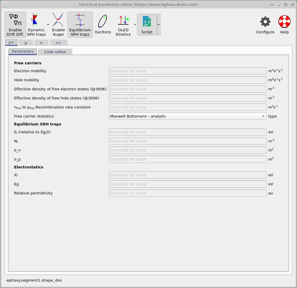
Clicking the Script button enables material scripting
??.
Parameters supplied by the script are then replaced in the editor by “See script for value”. Parameters whose corresponding Lua functions are disabled continue to use the fixed values stored in sim.json. This allows a script to control only the properties that need to be scripted while leaving all other parameters unchanged.
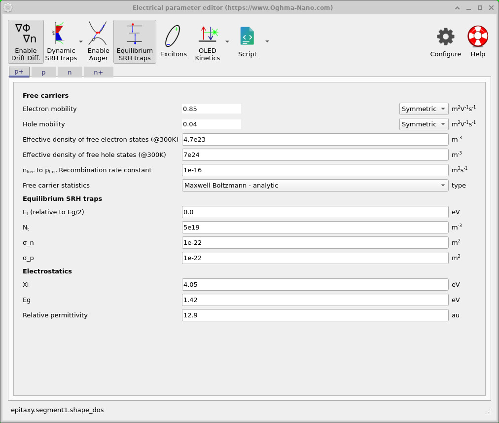
sim.json and the script is not used.
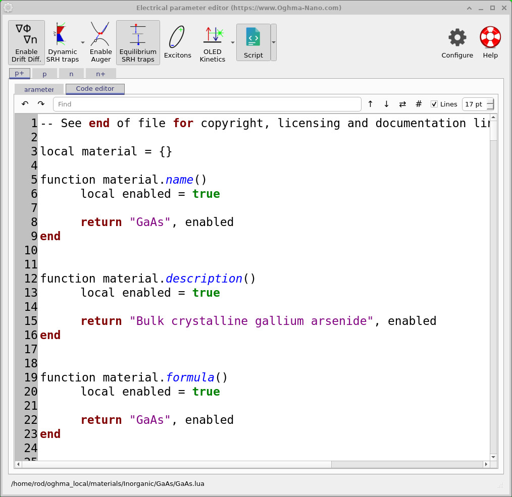
GaAs.lua).
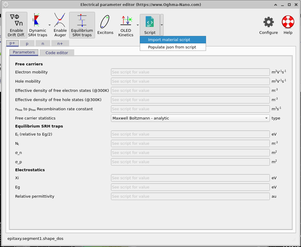
sim.json.
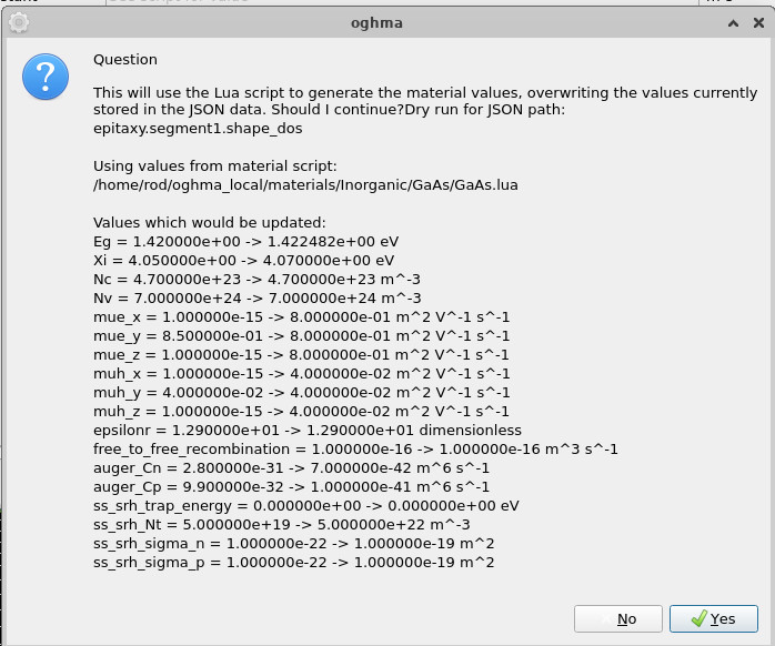
sim.json, listing every value that would change.
When scripting is enabled, a Code editor tab appears alongside the Parameters tab ??. This lets you inspect and edit the Lua material script directly from within the simulation without returning to the Materials database.
6.1 Selecting a script or copying its values into the simulation
The small menu beside the Script button provides two different ways of using a material script ??:
- Import material script — opens the Materials database and allows you to select the Lua material script that the simulation should use.
-
Populate json from script — evaluates the selected script and copies the resulting parameter values into the corresponding fixed values in
sim.json.
These two approaches serve different purposes. If the script is used directly, its functions remain active during the simulation. This is the appropriate mode when a parameter needs to vary with quantities such as temperature, position, composition, or photon density.
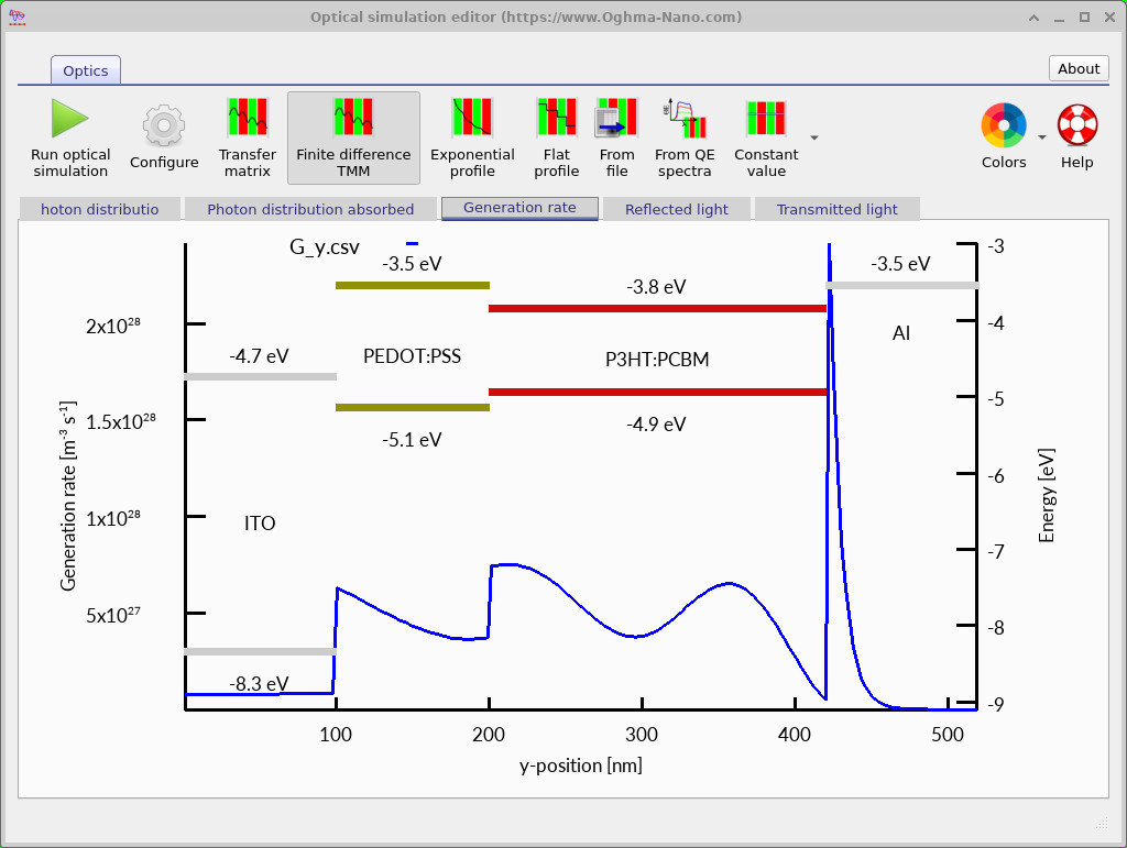
Eg and Xi are reflected here automatically.
Alternatively, Populate json from script can be used when you want the script to provide a well-defined set of starting values, but do not need the script to remain active. OghmaNano evaluates the script, writes the resulting numbers into the ordinary parameter fields, and those values can then be edited manually in the usual way.
Because populating sim.json can overwrite values already present in the simulation, OghmaNano first displays a confirmation dialog
??.
The dialog lists the script being used and shows each parameter that would change, together with its existing and proposed value. No values are changed until the operation is confirmed.
Two ways to use the same material script: keep the script active when parameters need to vary during the simulation, or use Populate json from script to obtain a set of fixed starting values that can subsequently be edited through the normal graphical interface.
7. Where the script's values are used
Values produced by a material script are used throughout the model, not just in the electrical solver. Quantities such as
Eg and Xi set the band-edge positions everywhere they are needed. For example, the energy levels drawn
in the band-diagram / generation-rate viewer are taken from these values
??. Editing the band
gap or affinity in a script therefore propagates automatically to the band diagram, the optical model, and the electrical
solver.
Common pitfalls
- The
local material = {}declaration must appear within the first 1000 bytes of the file, or OghmaNano will not recognise it as a material script. - Each function must return two values — the quantity and the
enabledflag. A box only reads “See script for value” when its function isenabled. - Work in SI units throughout (m, m-3, m2 V-1 s-1, eV as noted). Do a ballpark magnitude check on the values — do they make sense?
- Populate json from script overwrites the fixed values in
sim.json. Read the confirmation dialog before accepting.
Summary & next steps
- A Lua material script defines properties as functions of temperature, position, composition, or photon density; it is optional and only needed for varying or well-sourced parameters.
- Files are recognised by
local material = {}within the first 1000 bytes, and can live inside a material folder (shown with the material) or stand-alone (shown as a.luafile). - One electrical script commonly serves several optical (n/k) datasets; the model selects the most appropriate file and searches backwards when no script is present at the material level.
- In a simulation, the Electrical parameter editor can use fixed
sim.jsonvalues or a script; Populate json from script lets you pull script values into the fixed boxes. - Values such as
EgandXiare used throughout the model, including the band diagram.
Next: Return to Part C on how the database is stored, or see Optical database and Downloading more materials.