Lua scripting of the electrical Newton solver in OghmaNano

1. Introduction

OghmaNano includes an embedded Lua scripting interface that allows the internal numerical solver to be modified at runtime. This enables advanced control, such as enabling or disabling equations, altering the 3D Newton solver, freezing selected physics during transients or J–V scans, or implementing custom iterative strategies.

This is distinct from external scripting. Languages such as Python operate by modifying sim.json and launching the solver, making them well suited to parameter sweeps, batch execution, and post-processing.

In contrast, Lua operates inside the solver, allowing direct intervention in the numerical workflow without modifying the underlying C code.

2. What is Lua?

Lua is a lightweight, high-performance scripting language designed to be embedded inside larger applications. It is widely used in areas such as game engines and scientific software, where internal behaviour needs to be modified without recompiling the core code. Compared to Python, Lua has a much smaller footprint and lower runtime overhead, making it better suited to execution inside performance-critical loops. Compared to C, it is significantly easier to write and modify, while still providing fine control over program behaviour. These properties make Lua particularly well suited to OghmaNano, where it is used to directly influence the numerical solver during runtime.

Just to give you a feeling for Lua, if you have not programmed it before, here is an implementation of the classic bubble sort.

a = {5, 3, 8, 1, 2}
n = #a
for i = 1, n do
  for j = 1, n - i do
    if a[j] > a[j+1] then
      a[j], a[j+1] = a[j+1], a[j]
    end
  end
end

2. Accessing the Lua scripting editor

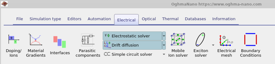
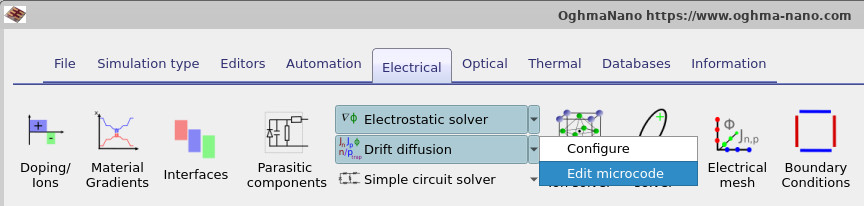
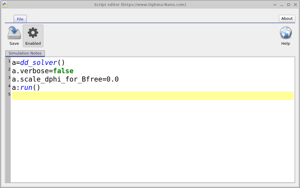
The Lua scripting editor can be accessed from the electrical ribbon of the main window, as shown in ??. Click on the small dropdown arrow next to the drift-diffusion solver control to open the menu, which is shown in ??. Then click on Edit microcode to open the Lua editor, which is shown in ??.

Press Ctrl+S to save the script, or use the save button in the editor toolbar. To enable the microcode, the enable button must be depressed, as shown in ??.

3. A simple example - a provskite solar cells with frozen ions

A simple example of using Lua scripting is in the simulation of perovskite devices, where one may want to freeze the mobile ions during a J–V scan. Perovskites contain mobile ions which drift relatively slowly. Experimentally, a device is often first held at a negative bias so that the ions move into a particular configuration, and then a very fast J–V scan is performed before they have time to respond significantly.

In OghmaNano, when the perovskite ion model is enabled, the electrical solver will normally allow the ions to relax at each voltage step. This is equivalent to a very slow or quasi-steady-state J–V scan. That is useful in some cases, but it does not reproduce experiments where the voltage is swept much more quickly. To mimic this type of measurement, the Lua script below can be used to freeze the ions when the main electrical loop begins. The simulation can still ramp to the required starting voltage in the normal way, allowing the ions to move during preparation, but once the main loop is entered the ion equation is disabled.

-- Initialise solver
a = dd_solver()
a.verbose = false              -- Suppress solver output

-- Apply logic only in the main electrical loop
if (a.problem_type & ELEC_PROB_MAIN_LOOP) ~= 0 then
    a.solve_nion = false       -- Disable ion equation (freeze ions)
    print("ion solver off")
else
    print("ion solver on")     -- Keep ions active during initialisation
end

a:run()                        -- Execute solver step

In this example, the solver object is first created and diagnostic output is reduced. The script then checks whether the current solver stage corresponds to the main electrical loop. If it does, the mobile ion equation is turned off by setting solve_nion=false, and the solver is then run with that modified equation set. There is an example simulation employing in the examples included with the model under "Perovskite cells/Perovskite solar cell - frozen ions (MAPI)".

5. Example: ADI scanning (Alternating-Direction Implicit)

A more advanced example of Lua scripting is the implementation of an alternating-direction strategy for solving complex three-dimensional problems. This approach is closely related to the Alternating-Direction Implicit (ADI) method, in which a multidimensional problem is decomposed into a sequence of lower-dimensional solves.

In OghmaNano, this idea can be implemented directly at the solver level by selectively enabling and disabling directional couplings. Rather than solving the fully coupled 3D system in one step, the domain is swept in alternating directions. This can significantly improve stability and convergence for difficult 3D drift–diffusion problems.

The strategy used here is to split the 3D problem into directional passes. In the first pass, the solver operates in x-slices, solving the full extent in y and z while removing the x-direction couplings. In the second pass, the solver switches to z-slices and performs the complementary operation. The total error is accumulated and used to define a custom convergence criterion.

The example below illustrates how such an ADI-style scan can be constructed using Lua:

-- Initialise solver and control variables
a = dd_solver()
cont = true
count = 0

-- Main ADI-style iteration loop
while cont == true do

-- ===== X-slice pass =====
a.set_newton_state("x")      -- Use/store Newton state for x-pass
tot_error = 0.0

a.step_z = -1                -- Full domain in z
a.step_x = 1                 -- Slice-by-slice in x
a.step_y = -1                -- Full domain in y

a.solve_pos_x = false        -- Disable x-direction Poisson coupling
a.solve_pos_y = true
a.solve_pos_z = true

a.solve_je_x = 0             -- Disable x-direction electron current
a.solve_jh_x = 0             -- Disable x-direction hole current
a.solve_je_y = true
a.solve_jh_y = true
a.solve_je_z = true
a.solve_jh_z = true

a.solve_srh_e = true         -- Keep SRH recombination active
a.solve_srh_h = true

a.solve_nion = 0             -- Disable ions
a.solve_singlet = false      -- Disable excited-state physics

error = a:run()              -- Execute x-slice solve
tot_error = tot_error + error


-- ===== Z-slice pass =====
a.set_newton_state("z")      -- Switch to z-pass Newton state

a.step_z = 1                 -- Slice-by-slice in z
a.step_x = -1                -- Full domain in x
a.step_y = -1                -- Full domain in y

a.solve_pos_x = true
a.solve_pos_y = true
a.solve_pos_z = false        -- Disable z-direction Poisson coupling

a.solve_je_y = true
a.solve_jh_y = true
a.solve_je_x = true
a.solve_jh_x = true
a.solve_je_z = false         -- Disable z-direction transport
a.solve_jh_z = false

a.solve_srh_e = true
a.solve_srh_h = true
a.solve_nion = false
a.solve_singlet = false

error = a:run()              -- Execute z-slice solve
tot_error = tot_error + error


-- ===== Convergence logic =====
if (error < 1e-3) then       -- Local convergence check
    if (count > 2) then      -- Ensure minimum iterations
        cont = false
    end
end

print("count", count, "tot error:", error)

count = count + 1

if (tot_error < 1e-7) then   -- Global convergence criterion
    cont = false
end

if (count > 10) then         -- Safety iteration limit
    cont = false
end

end

In this implementation, two directional passes are performed within each iteration. The first pass disables x-direction Poisson and carrier transport terms, effectively solving the system slice-by-slice along x. The second pass disables the corresponding z-direction terms, producing a complementary sweep.

Separate Newton states are maintained for each directional pass using set_newton_state(), allowing the solver to retain independent internal variables such as electrostatic potential, carrier densities, and trap occupancies.

Convergence is controlled explicitly in the Lua script. The loop terminates when either the per-pass error and iteration count satisfy a threshold condition, the accumulated error falls below a specified tolerance, or a maximum number of iterations is reached.

This example illustrates how Lua scripting can be used to construct fully custom solver workflows. Rather than relying on a fixed numerical scheme, the user can directly define how the multidimensional system is decomposed, how intermediate states are managed, and how convergence is assessed. This is particularly valuable for complex 3D simulations where fully coupled approaches may be unstable or computationally inefficient.

3. The dd_solver() object

The entry point for Lua control of the electrical solver is the dd_solver() object. This provides direct access to the internal drift–diffusion/Newton solver, allowing both the equation set and the solution strategy to be modified at runtime.

In practical terms, the solver object enables three core operations:

1. Inspect the current solver context (e.g. problem type or applied bias).
2. Enable or disable individual equations and directional couplings.
3. Execute a solver step and retrieve a convergence/error metric.

The most commonly used fields are summarised in Table ??.

In addition to field access, the solver exposes a small number of key methods:

8. Summary

Lua scripting in OghmaNano provides direct control over the internal drift–diffusion solver, enabling the user to modify the mathematical system being solved at runtime. Unlike external scripting approaches, which operate on input files, Lua acts within the solver loop itself and can therefore alter equation sets, directional couplings, and convergence behaviour on a step-by-step basis. This capability is particularly valuable in situations where the standard fully coupled formulation is either not physically appropriate or numerically efficient. Examples include freezing slow degrees of freedom such as mobile ions, or decomposing complex 3D problems into directional passes using ADI-style strategies.

The examples presented here illustrate two key use cases. The first demonstrates a minimal intervention, where the ion equation is disabled only in the main electrical loop to reproduce fast-scan experimental conditions. The second shows how Lua can be used to construct a custom solver workflow, alternating between directional slices and applying user-defined convergence criteria.

More generally, Lua should be viewed as a framework for numerical method development within OghmaNano. It allows the user to move beyond fixed solver configurations and instead define tailored solution strategies that are aligned with both the physics of the problem and the numerical properties of the system being solved.