OghmaNano contains an advanced Finite-Difference Time-Domain (FDTD) solver for modelling electromagnetic wave propagation in the time domain. The solver is designed for problems in integrated photonics, waveguide optics, resonators, interference, diffraction, and general structured optical systems. Because the fields are solved directly on a spatial grid as a function of time, the method naturally captures propagation delay, scattering, reflection, interference, cavity build-up, and transient response within one unified framework.
The same FDTD framework can be applied to a wide range of optical structures, including free-space propagation problems, photonic crystal waveguides, ring resonators, Mach–Zehnder devices, and double-slit interference simulations. Because the solver works directly in the time domain, it is particularly useful for studying pulse propagation, detector delay, resonant energy build-up, and the dynamic response of optical systems to different excitation waveforms.
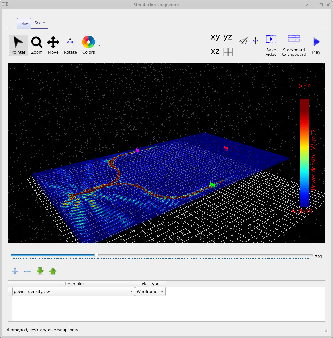
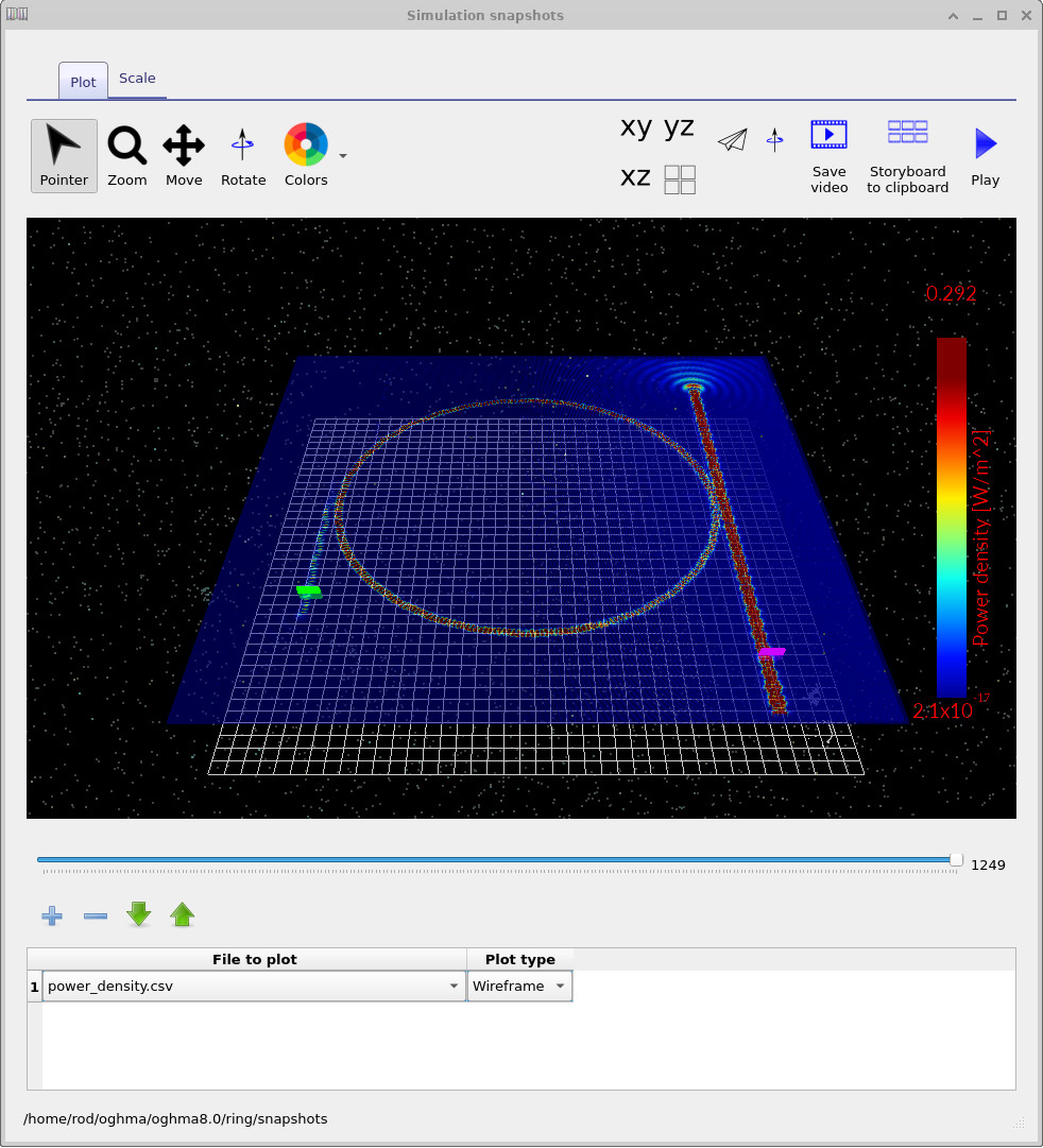
The user can define time-domain light sources, assign boundary conditions, place detectors, and inspect power-density snapshots throughout the simulation. In practice this makes it possible to move from a simple teaching example to a more realistic photonic device while staying within the same workflow and using the same solver engine.
The FDTD solver advances Maxwell’s curl equations directly in time on a discretised spatial mesh. In source-free form these are
$$ \mu \frac{\partial \mathbf{H}}{\partial t} = - \nabla \times \mathbf{E} $$ $$ \varepsilon \frac{\partial \mathbf{E}}{\partial t} + \sigma \mathbf{E} = \nabla \times \mathbf{H} $$In the numerical scheme, the electric and magnetic fields are staggered in both space and time so that the fields are updated explicitly from one time step to the next. This makes the method well suited to transient optical simulations where the goal is to observe how a pulse or continuous-wave excitation evolves as it interacts with a complex structure.
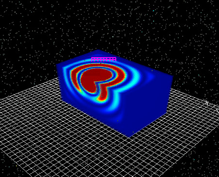
Because the fields are solved directly rather than reduced to a frequency-domain steady-state problem, the method naturally resolves effects such as resonance build-up, delayed detector response, transient scattering, and the time-dependent evolution of power flow. This is one of the main reasons FDTD is such a useful tool for photonics and wave-optics modelling.
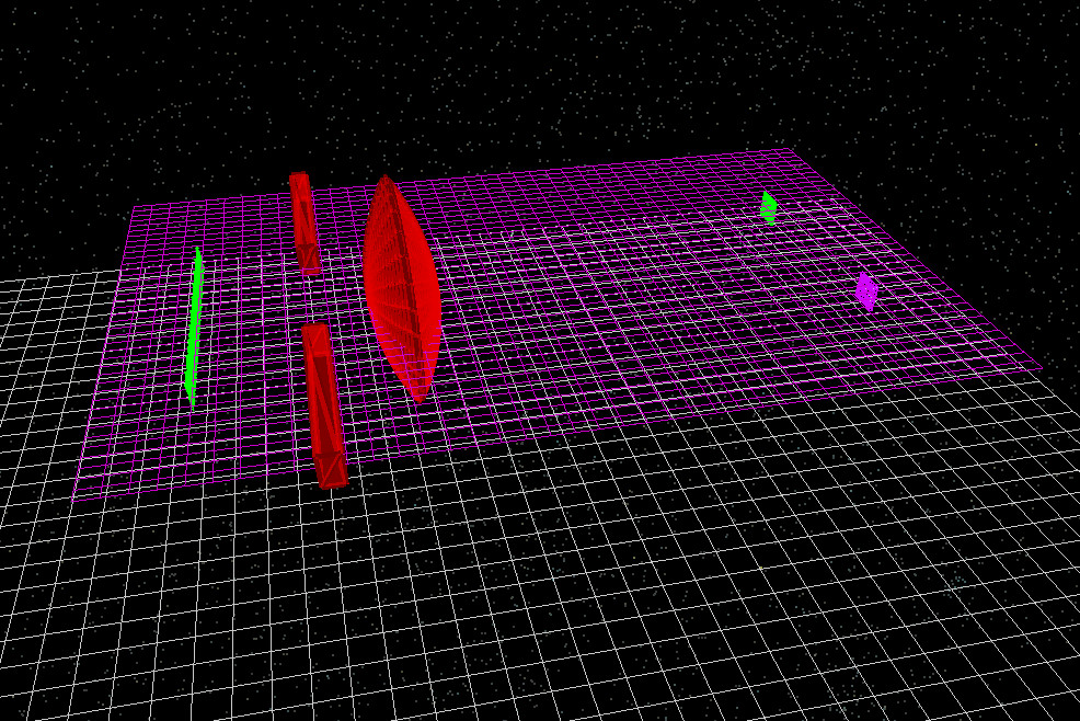
Every FDTD simulation depends on three core ingredients: how the field is launched, how the outer edges of the domain are treated, and how the response is measured. OghmaNano includes dedicated editors for each of these. Time-domain excitation is defined through the FDTD light source settings, where the user can select continuous-wave or pulsed excitation, control the injected field components, and adjust timing and waveform parameters.
The outer edges of the simulation region are controlled through the boundary-condition editor. Depending on the problem, the user can choose absorbing boundaries such as PML, simpler absorbing conditions such as Mur ABC, or periodic boundaries for repeated structures. In practice this determines whether waves leave the domain cleanly, reflect from the outer edge, or repeat across opposite faces of the simulation box.
Detectors then record the time-dependent response of the device. These can be used to monitor transmitted power, coupled power, delay, and transient build-up in resonant structures. The combination of sources, boundary conditions, and detectors is what turns the solver from a field visualiser into a practical photonic device-analysis tool.
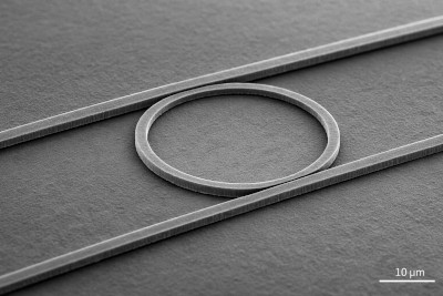
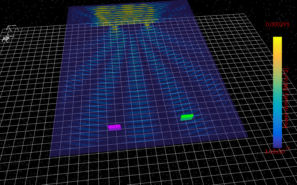
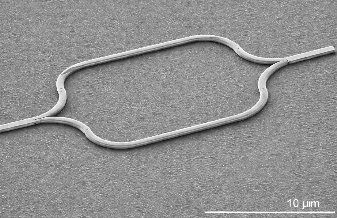
The FDTD solver can be used for a broad range of wave-optics problems. In integrated photonics it can model ring resonators, directional couplers, Mach–Zehnder devices, photonic-crystal waveguides, and other on-chip optical circuits. In teaching and interference problems it can simulate free-space propagation, diffraction, and double-slit interference. More broadly, it can be used wherever the time evolution of the electromagnetic field matters.
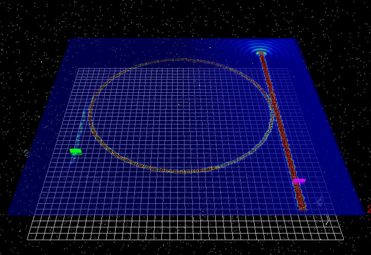
Because the method is solved directly in time, it is especially useful when the user wants to understand not only what the final field pattern looks like, but how it forms. That includes pulse transit, resonator ring-up and ring-down, scattering from structured boundaries, and detector delay between different optical paths. In structures such as the ring resonator shown in Figure ?? and Figure ??, the time-domain viewpoint is often the most intuitive way to understand the underlying physics.
The solver is also a useful bridge between idealised photonic concepts and more realistic structures. Structured optical geometries, integrated devices, and even more complex optical assemblies can be explored in the same environment, provided they can be represented on the simulation grid. This makes the FDTD module valuable both for research problems and for tutorial-style examples that build physical intuition.
OghmaNano includes a growing set of example FDTD simulations and step-by-step tutorials. These are a good way to move quickly from the underlying method to practical device problems. The examples cover both introductory wave-optics problems and more structured integrated-photonics geometries.
Useful starting points include the free-space green-light propagation example, the double-slit interference tutorial, the photonic crystal waveguide tutorial, the ring resonator tutorial, and the silicon Mach–Zehnder modulator example. Taken together, these examples show how the same solver can be used for propagation, interference, resonance, coupling, and time-domain detector analysis.
Try an FDTD example.
Start with the free-space propagation tutorial for a first look at the method, then move on to ring resonators, Mach–Zehnder devices, or photonic crystal waveguides.
For the underlying theory, see the FDTD theory page, FDTD light sources, and FDTD boundary conditions.