FDTD tutorial: Free-space propagation of green light

1. Overview: what you will simulate

This tutorial introduces the Finite-Difference Time-Domain (FDTD) engine in OghmaNano using the simplest possible physical system: electromagnetic wave propagation in free space. A monochromatic source of green light, with a wavelength between 531 nm and 532 nm, is launched into an empty computational domain. There are no waveguides, no resonators, and no materials other than vacuum. The purpose is not to demonstrate a device, but to make the numerical machinery visible.

The FDTD module solves Maxwell’s curl equations directly in the time domain on a discrete spatial grid. At each time step, the electric and magnetic fields are updated across the entire mesh. Because the algorithm is highly parallel, OghmaNano executes it using OpenCL and will automatically use your GPU if one is available. This tutorial therefore serves as both a physics demonstration and a first introduction to the GPU-accelerated FDTD backend.

By the end of this page you will have created a simulation, inspected the world size and spatial mesh, run the solver, and visualised how green light propagates through space in three dimensions.

2. Creating the Free space simulation

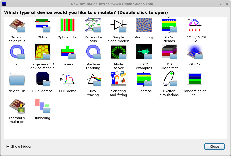
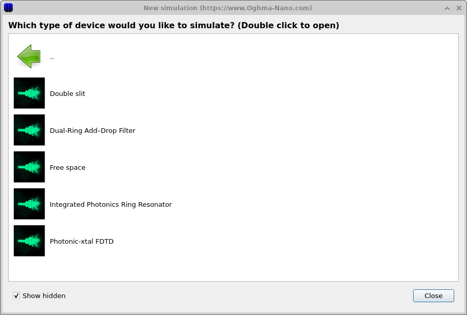
Open the New simulation window and select the FDTD examples category, then choose the example called Free space. The two selection windows are shown below.

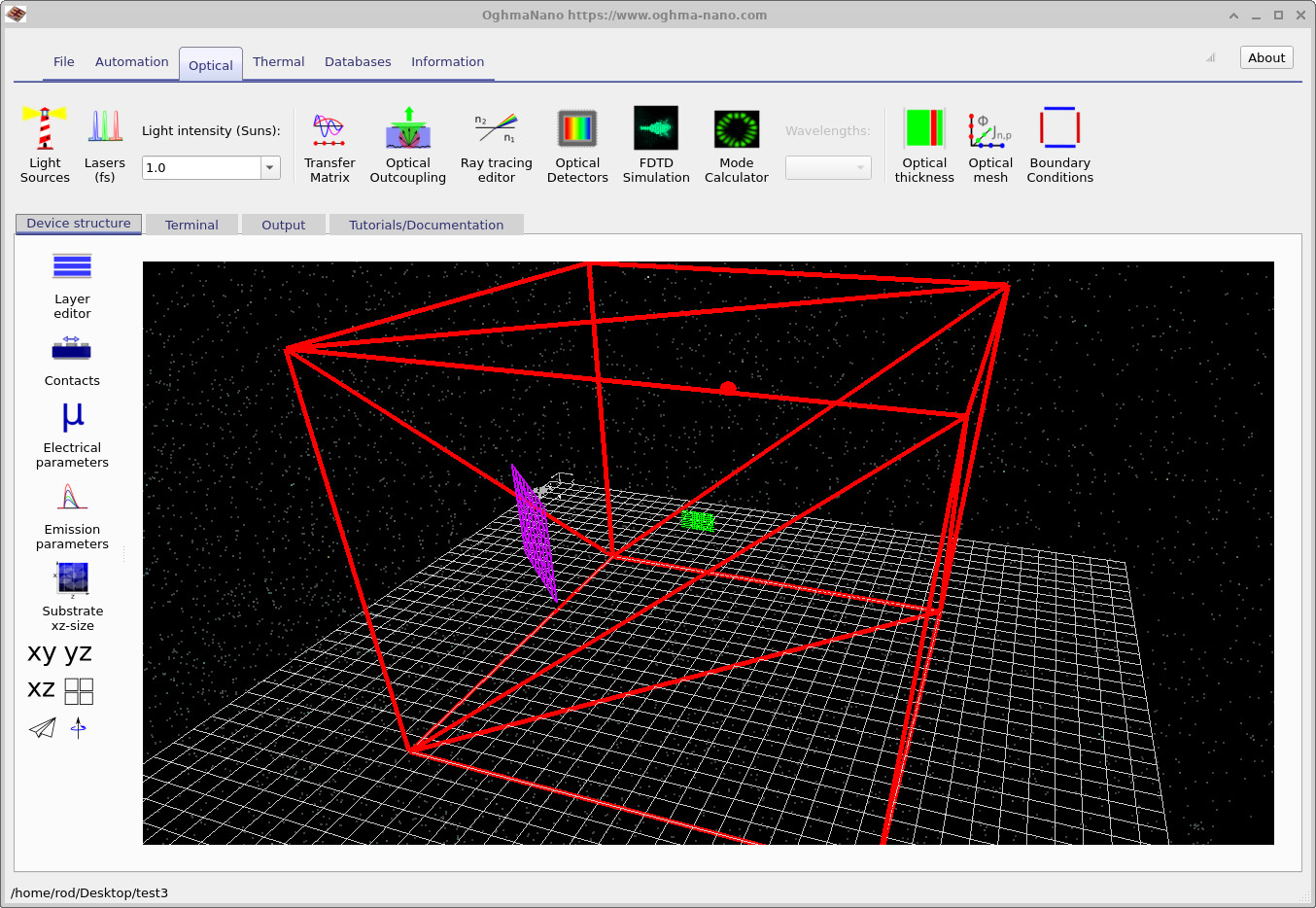
New simulation window showing the FDTD examples category. — Open *FDTD examples* from the New simulation window.

FDTD example list showing the Free space simulation. — Select the **Free space** example.

After loading, the main OghmaNano window appears with a simple three-dimensional scene. The computational world is initially empty except for a source and a detector region. Right-click inside the 3D view and enable Show world box. A red bounding box will appear, defining the limits of the FDTD domain.

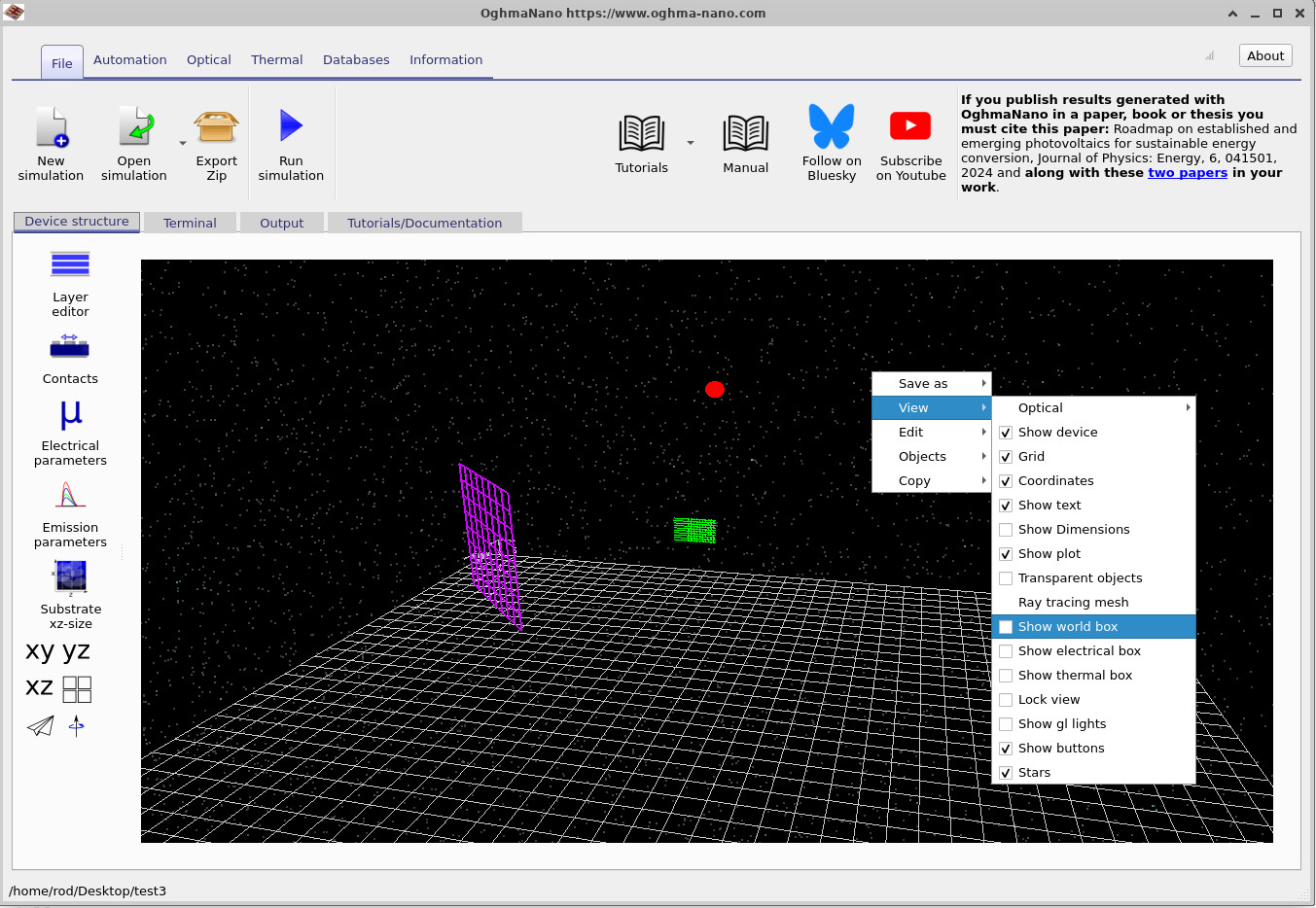
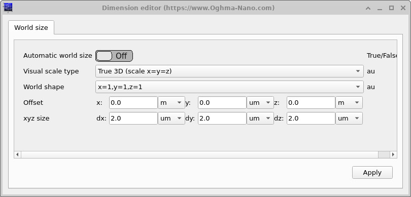
Main OghmaNano window showing the Free space simulation with a visible world box. — The main window with the simulation domain visible.

World size editor showing the dimensions of the FDTD simulation domain. — The world size editor, accessed via the *Substrate xz-size* button.

The world dimensions can be inspected by clicking the Substrate xz-size button on the left-hand toolbar. This opens the world size editor, where the physical size of the simulation domain is defined in micrometres. For this tutorial you do not need to change anything; the domain has already been configured to comfortably contain several wavelengths of green light.

3. Inspecting the optical settings and mesh

Next, open the Optical ribbon at the top of the window.

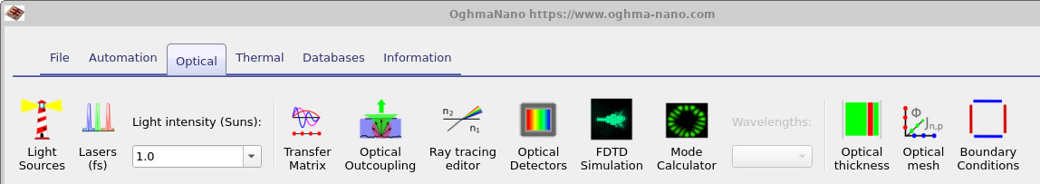
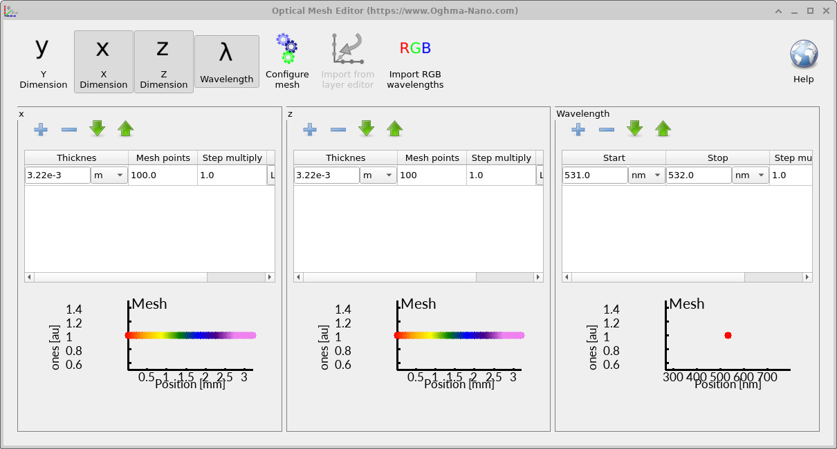
Optical ribbon in OghmaNano showing the Optical mesh button. — The Optical ribbon. Click **Optical mesh** to inspect the spatial discretisation.

Click Optical mesh to open the mesh editor.

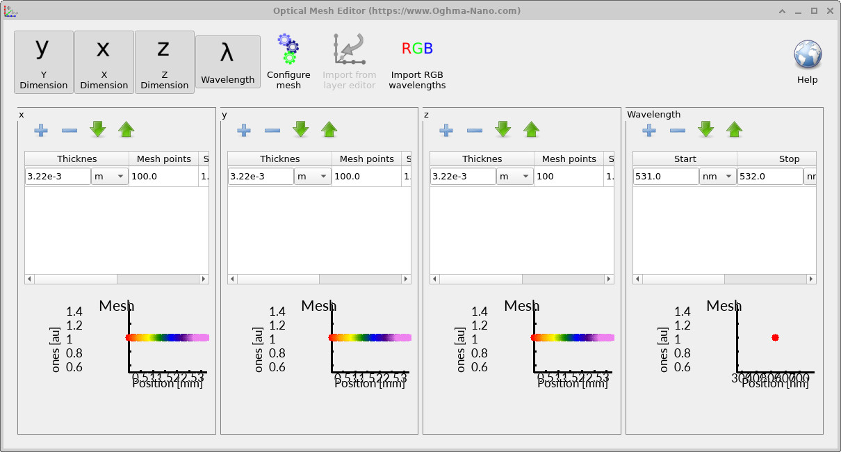
Optical mesh editor showing mesh points and wavelength range between 531 nm and 532 nm. — Optical mesh settings, including spatial resolution and wavelength range (531–532 nm).

The mesh editor displays how many grid points are used in each spatial direction. These determine the spatial resolution of the FDTD calculation. The wavelength range is set between 531 nm and 532 nm, which corresponds to green light. In this example, the thickness parameters shown in the mesh editor are automatically scaled to the world size and can be ignored. The important point is that the spatial grid is sufficiently fine to resolve the electromagnetic wavelength.

4. Running the GPU-accelerated FDTD solver

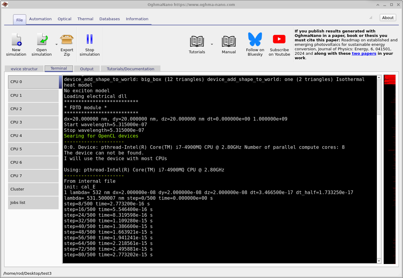
Start the simulation by clicking the Run simulation button or pressing F9. The Terminal tab will display solver information.

Terminal output showing FDTD run and the message Searching for OpenCL devices. — Terminal output during execution. The solver searches for OpenCL devices before launching.

In the Terminal output, notice the green text stating Searching for OpenCL devices. At this stage the program is scanning your system for compatible GPUs. On systems with a supported graphics card, the solver will select the GPU and run the time-stepping loop there. In the example shown, the calculation is running on a CPU backend emulating an OpenCL device, but on a modern workstation the same simulation will automatically use the graphics processor for acceleration.

5. Inspecting the output and field snapshots

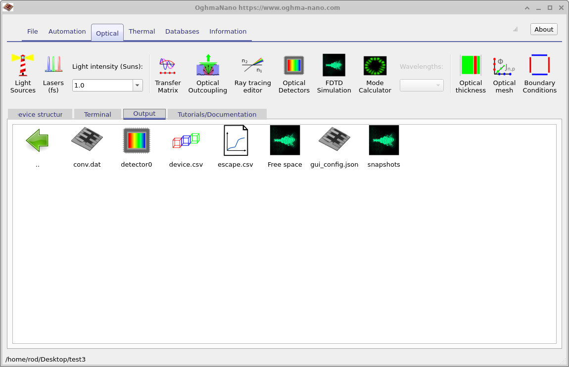
After completion, switch to the Output tab. The generated files are listed there.

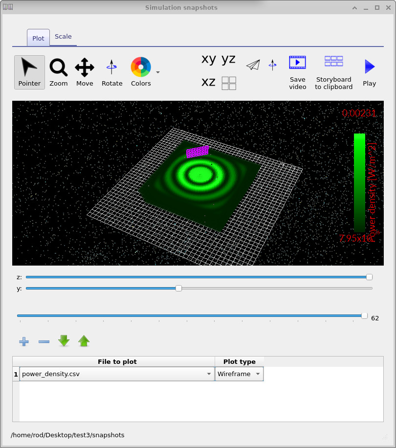
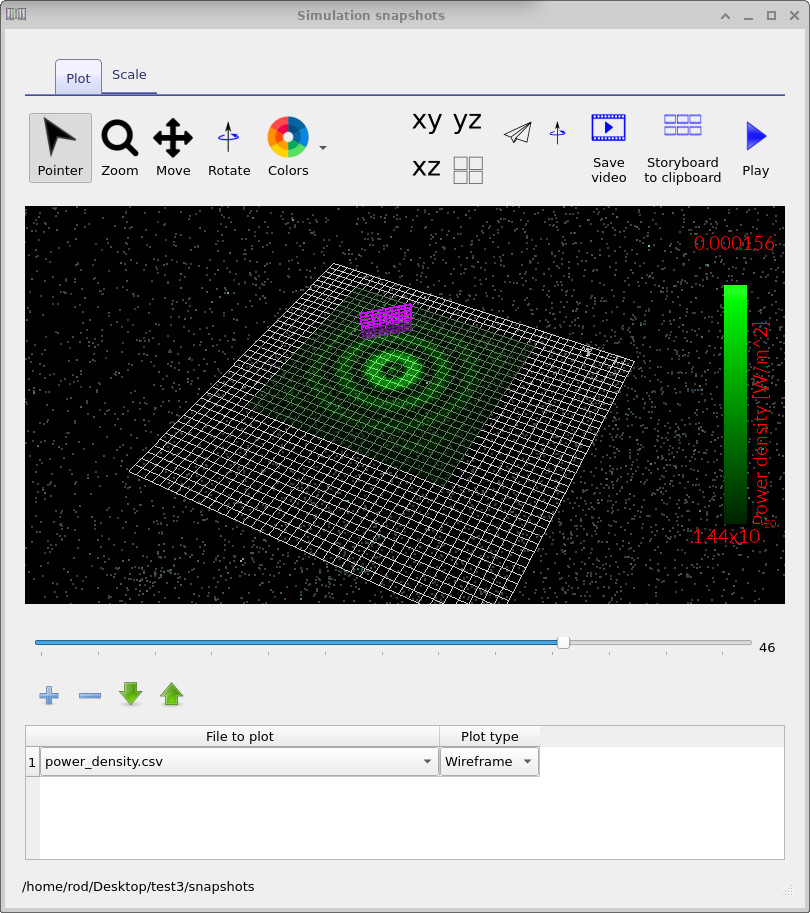
Output tab listing simulation results including the snapshots directory. — The Output tab after the simulation completes.

Snapshot viewer showing green light propagating in free space. — Snapshot viewer: select *power density* and use the sliders to explore time and space.

Double-click the snapshots directory to open the snapshot viewer. Select power density from the drop-down list at the bottom of the window. The coloured field represents the instantaneous electromagnetic energy density. Use the horizontal slider to move forward and backward in time, and the spatial sliders to examine different cross-sections of the domain. On some computers, especially when running large meshes, the viewer may take a short moment to respond as it loads each dataset.

Later-time snapshot showing spherical wavefront propagation. — A later-time snapshot showing outward propagation of the green-light wavefront.

As you step through time, you will observe the wavefront expanding across the domain. In free space, without boundaries or structures, the propagation is uniform and symmetric, limited only by the absorbing boundary conditions at the edges of the computational box.

6. Viewing detector power

The purple grid visible in the main window represents a detector plane placed inside the simulation domain. Double-click detector 0 in the Output tab to open its recorded power trace.

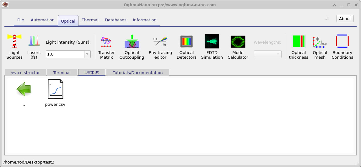
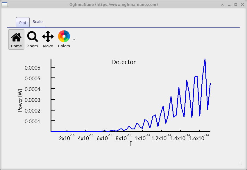
Main window showing the detector plane in purple. — The detector plane (purple grid) inside the free-space domain.

Detector power versus time plot. — Detector power as a function of time.

The resulting plot shows the electromagnetic power crossing that plane as a function of time. Initially the detector records zero signal. As the wavefront reaches the plane, the measured power rises and then stabilises according to the temporal profile of the source. This simple configuration makes it easy to connect the visual propagation of the wave in the snapshot viewer with a quantitative power measurement.

You have now completed your first FDTD simulation in OghmaNano. Although the system contained no materials or devices, it demonstrated the full numerical pipeline: world definition, mesh construction, GPU device selection, time stepping, field visualisation, and detector extraction. In subsequent tutorials, these same tools will be applied to structured photonic and optoelectronic systems.

7. Speeding up the simulation by switching to 2D (XZ)

Often, fully three-dimensional simulations are not necessary for understanding structures and devices, particularly when the physics is essentially invariant in one direction. In those cases you can obtain a considerable speed-up by reducing the problem to two dimensions. For the Free space example, switching from a 3D world to an XZ simulation removes the entire Y-dimension from the computational grid. The result is fewer mesh points, less field data, and dramatically shorter run times—typically fast enough that reruns become effectively interactive.

To do this, navigate back to the Optical ribbon, open Optical mesh, and select the 2D mesh configuration shown in ??. The key change is that the Y-axis is suppressed so the simulation becomes an XZ-plane calculation.

Optical mesh editor configured for a 2D XZ simulation by suppressing the Y dimension. — Optical mesh configured for 2D: suppress the Y-axis to run an XZ simulation.

Snapshot viewer in 2D showing the wave propagating in the XZ plane. — The snapshot viewer in 2D: the field evolution in the XZ plane renders quickly and is easy to scrub through.

FDTD editor showing output verbosity to disk set to write everything to disk. — For smoother playback, increase snapshot density by setting output verbosity to *Write everything to disk*.

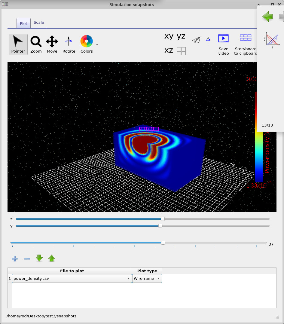
With the mesh now reduced to two dimensions, run the simulation again. You should immediately notice that the solver completes almost instantaneously compared to the 3D case. Open the snapshots/ directory again and scroll through time in the snapshot viewer (??). Because the dataset is much smaller, the viewer not only loads faster, it also responds more quickly when you drag the time slider or move the spatial cross-section controls.

One detail to be aware of is that the perceived smoothness of the animation can change. In the 2D run, the simulation advances very quickly and you are typically dumping fewer frames, so when you scrub through time the evolution may look slightly jerky—simply because there are fewer recorded snapshots between one time index and the next. If you want to follow the wave propagation in finer temporal detail, increase the amount of output written to disk.

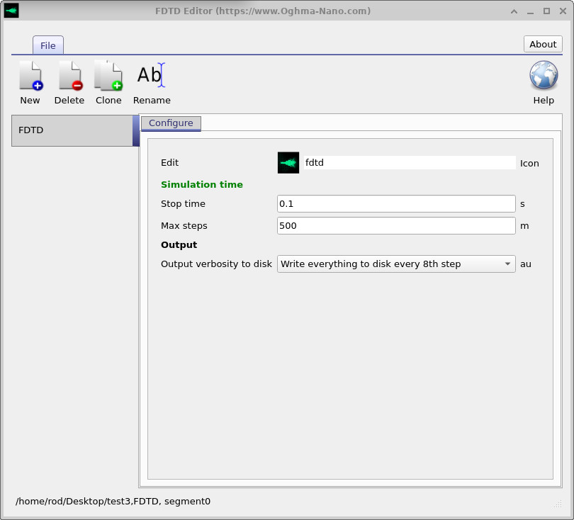
To do this, go again to the Optical tab, click the FDTD simulation button to open the FDTD configuration window, and change Output verbosity to disk from Write everything to disk every 8th step to Write everything to disk (??). This writes a snapshot every single time step. When you reopen the snapshot viewer, you will be able to follow the wave propagating over time very exactly, with much finer temporal resolution during playback and scrubbing.