Fabry–Pérot Cavity Simulation (FDTD): 1D Optical Resonator Tutorial
1. Introduction
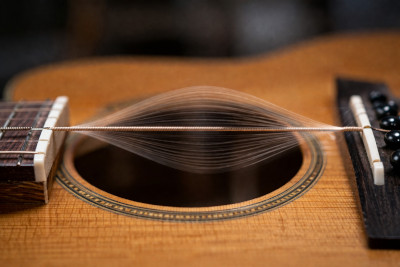
A Fabry–Pérot cavity is one of the most important resonant structures in optics and photonics. At its simplest, it is a region bounded by two reflecting surfaces, so that light can bounce back and forth and form standing-wave resonances. A familiar mechanical analogy is a vibrating guitar string, shown in ??. Just as only certain vibration patterns are allowed on a fixed string, corresponding to specific wavelengths and frequencies (musical notes), only certain optical modes are supported inside a Fabry–Pérot cavity.
The optical version of this idea is illustrated in ??. Light reflects repeatedly between two interfaces, and these multiple passes interfere with one another. When the round-trip phase is correct, the waves add coherently and a resonant mode builds up inside the cavity. This simple principle underpins a wide range of photonic devices, including optical filters, dielectric mirrors, interferometers, and laser cavities.
In a Fabry–Pérot resonator, only optical modes whose wavelength fits the cavity are allowed. At normal incidence, this occurs when the resonance condition is
\(2nL = m\lambda\)
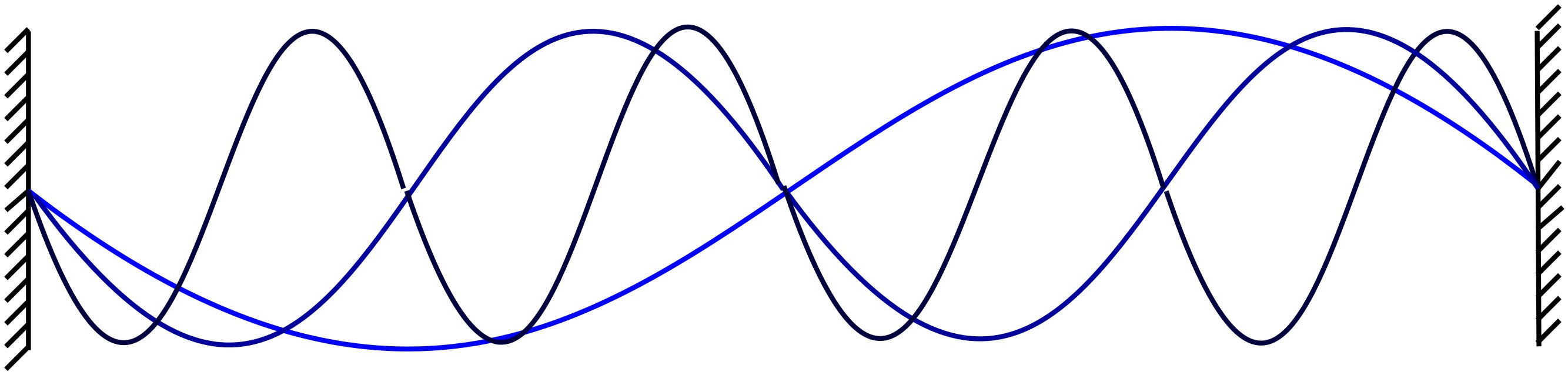
where \(n\) is the refractive index of the cavity region, \(L\) is the cavity length, \(\lambda\) is the wavelength, and \(m\) is an integer mode number. In the figure, three modes are shown: the fundamental mode (m = 1, light blue), the second harmonic (m = 2, blue), and the third harmonic (m = 3, dark blue). This means the cavity supports a discrete set of standing-wave solutions rather than an arbitrary continuum of wavelengths.
Equivalently, the allowed wavelengths may be written as
\(\lambda_m = \dfrac{2nL}{m}\)
Higher-order modes therefore correspond to different integer values of \(m\), each giving a different resonant field pattern. This is exactly the behaviour suggested by the standing-wave analogy and is the reason Fabry–Pérot cavities are widely used as optical resonators, wavelength-selective elements, and laser cavities.
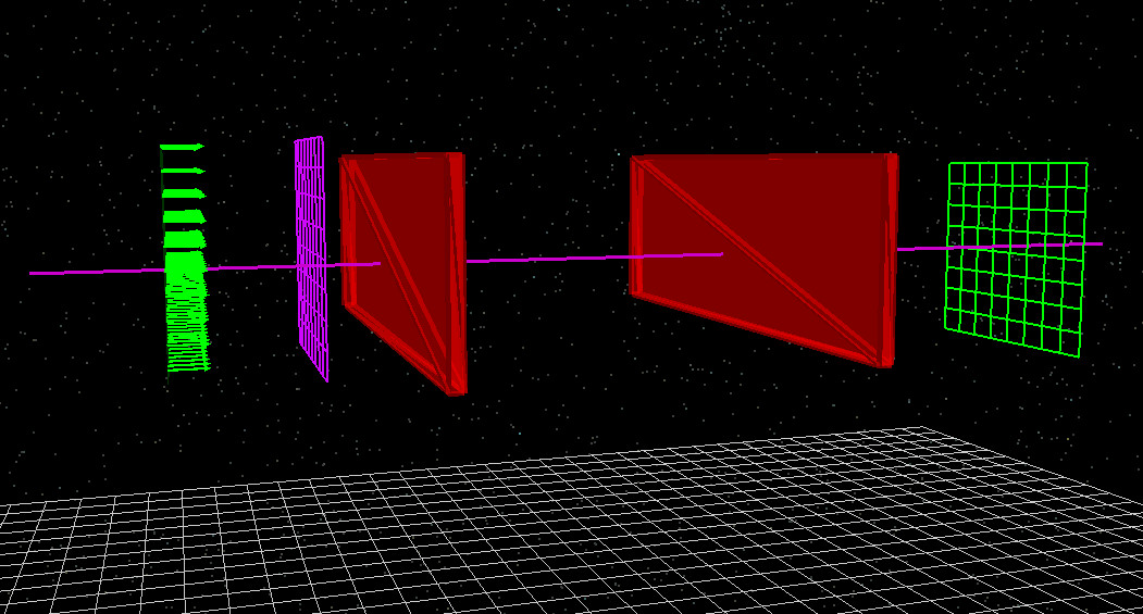
In this tutorial, we use the Finite-Difference Time-Domain (FDTD) method to simulate a simple 1D Fabry–Pérot cavity. The simulation contains a source, two reflecting regions, a cavity between them, and detector planes that record the optical response ( ??). By running this model, you will see how a broadband pulse excites the cavity, how standing waves form, and how the transmitted and reflected spectra reveal the resonant modes of the device.
2. Making a new simulation
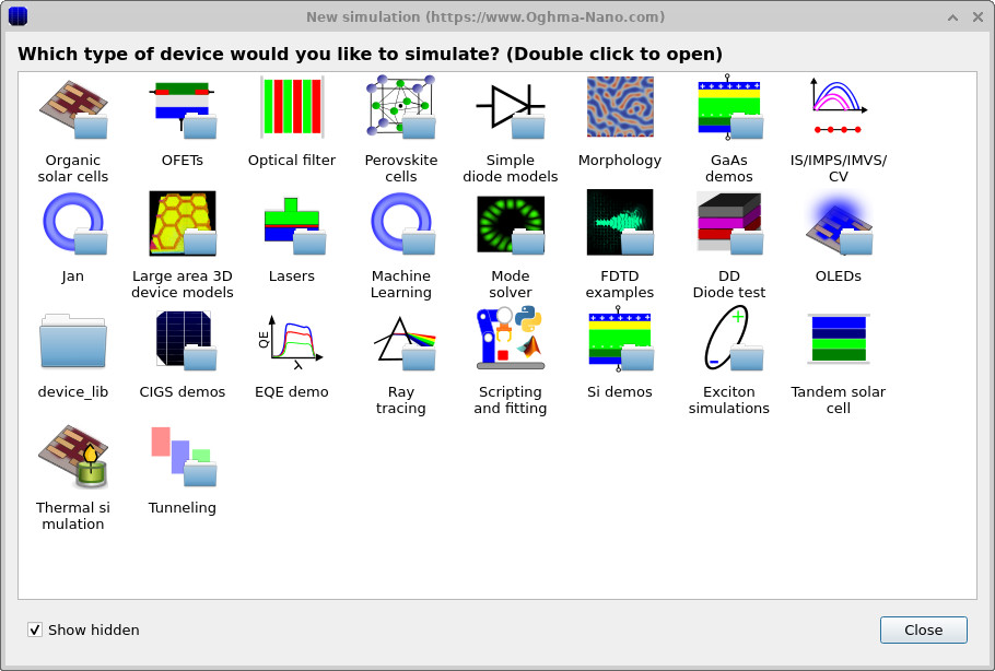
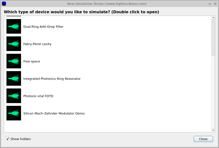
Open the New simulation window and select the FDTD examples category (??). Then choose the Fabry–Pérot cavity example (??). This loads the main interface shown in ??.
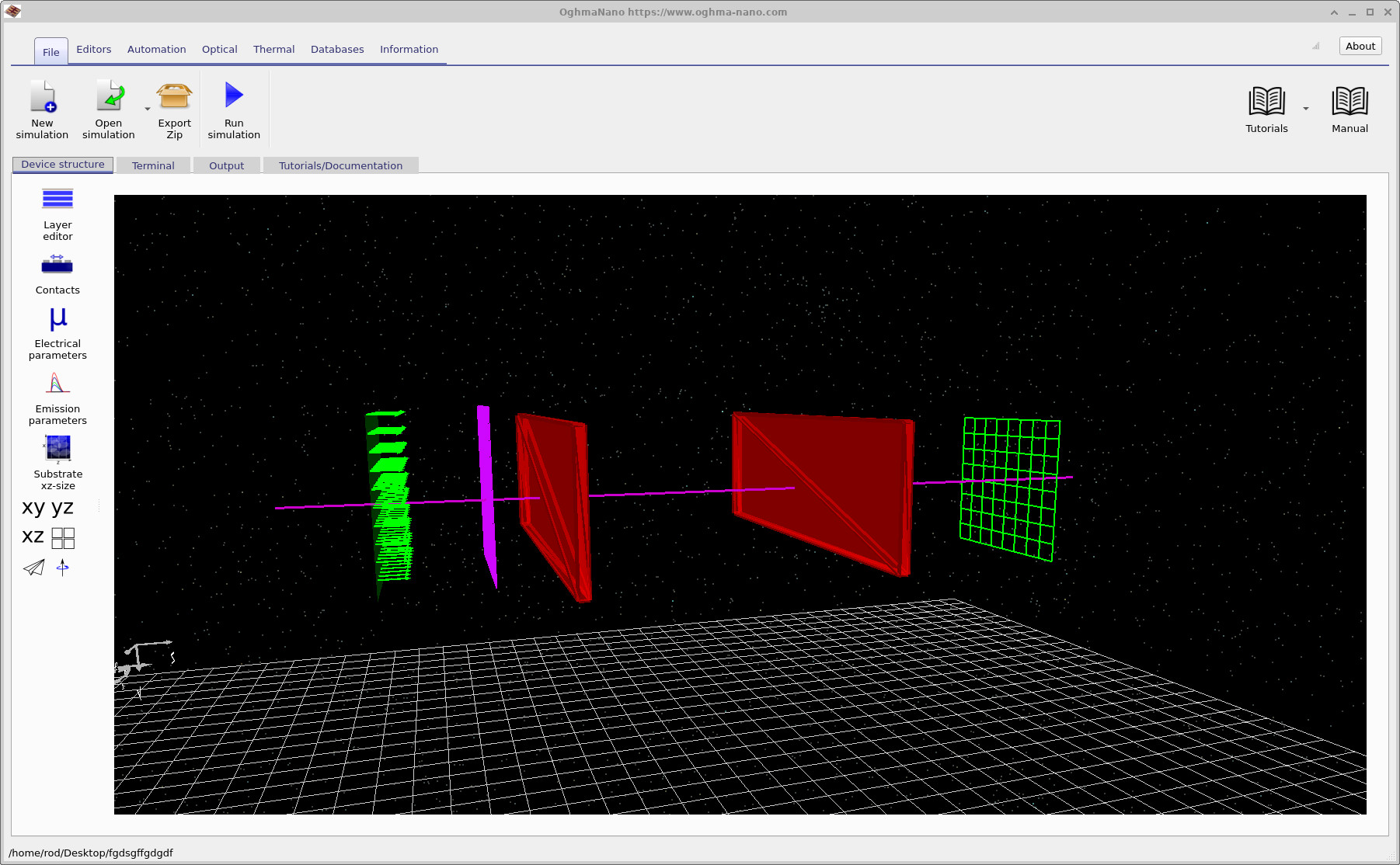
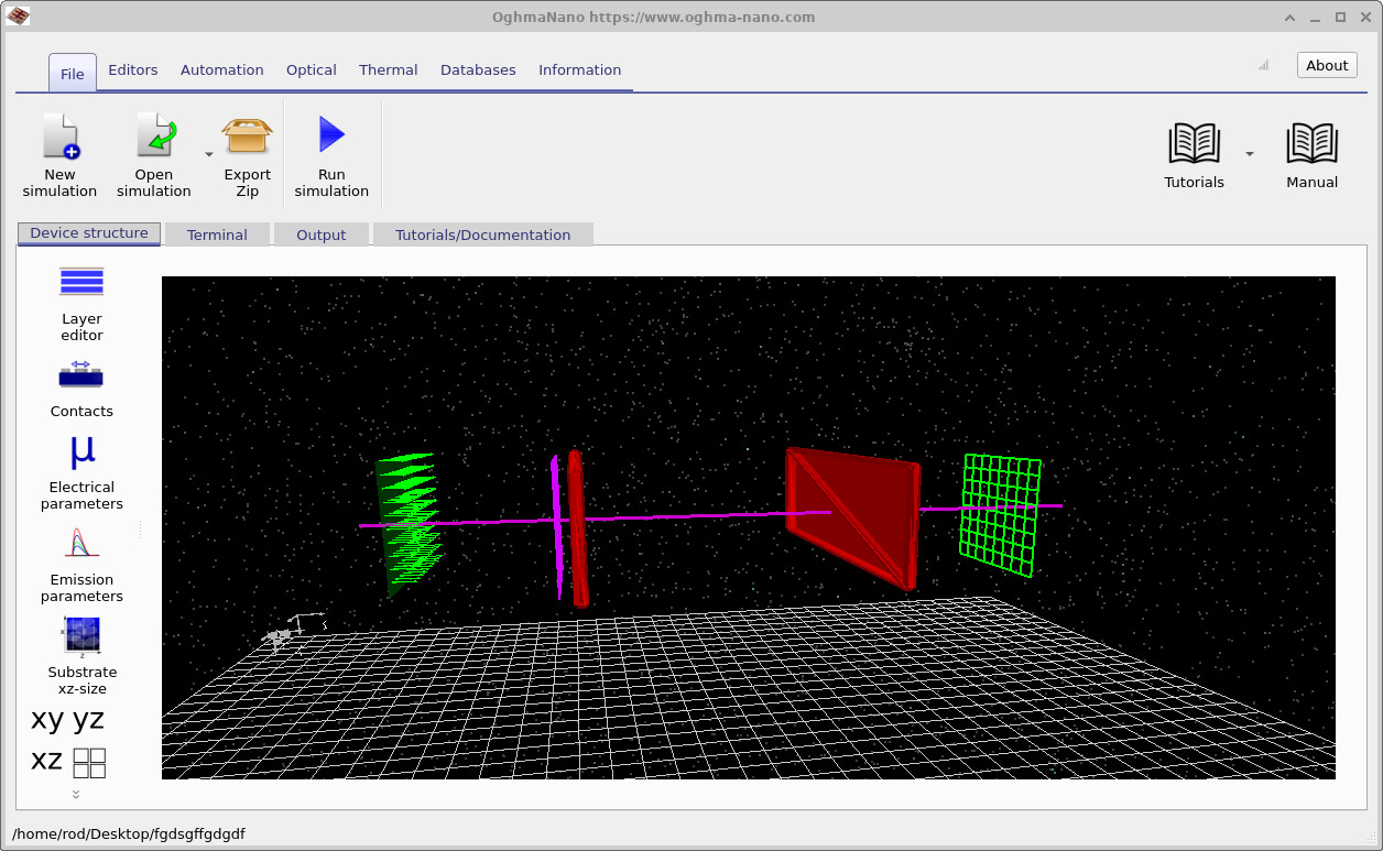
After loading the simulation, the main window appears as shown in ??. The structure is displayed in the 3D view within the Device structure tab. This view shows all the key components of the Fabry–Pérot cavity simulation.
On the left, the green arrows represent the FDTD source, where the optical pulse is injected. The thin purple line running through the structure is the FDTD grid. In this example, the simulation is effectively one-dimensional, so the grid appears as a single line passing through the cavity.
Just to the right of the source, the purple plane represents the input detector, which records the incoming and reflected fields. At the centre of the structure are the two reflecting regions that form the Fabry–Pérot cavity. On the right-hand side, the green plane is the output detector, which measures the transmitted light after it passes through the cavity. The detectors do not affect the propagation of the wave; they simply record the electromagnetic field as it evolves in time.
In a moment, we will run the simulation and observe how light travels through the structure and interacts with the cavity. You will see how the wave is partially reflected, how part of it enters the cavity and builds up between the mirrors, and how this behaviour is recorded by the two detectors on either side of the structure.
3. Running the simulation
Once you have saved the simulation and had a look around the structure, click the Run (▶) button to start the calculation.
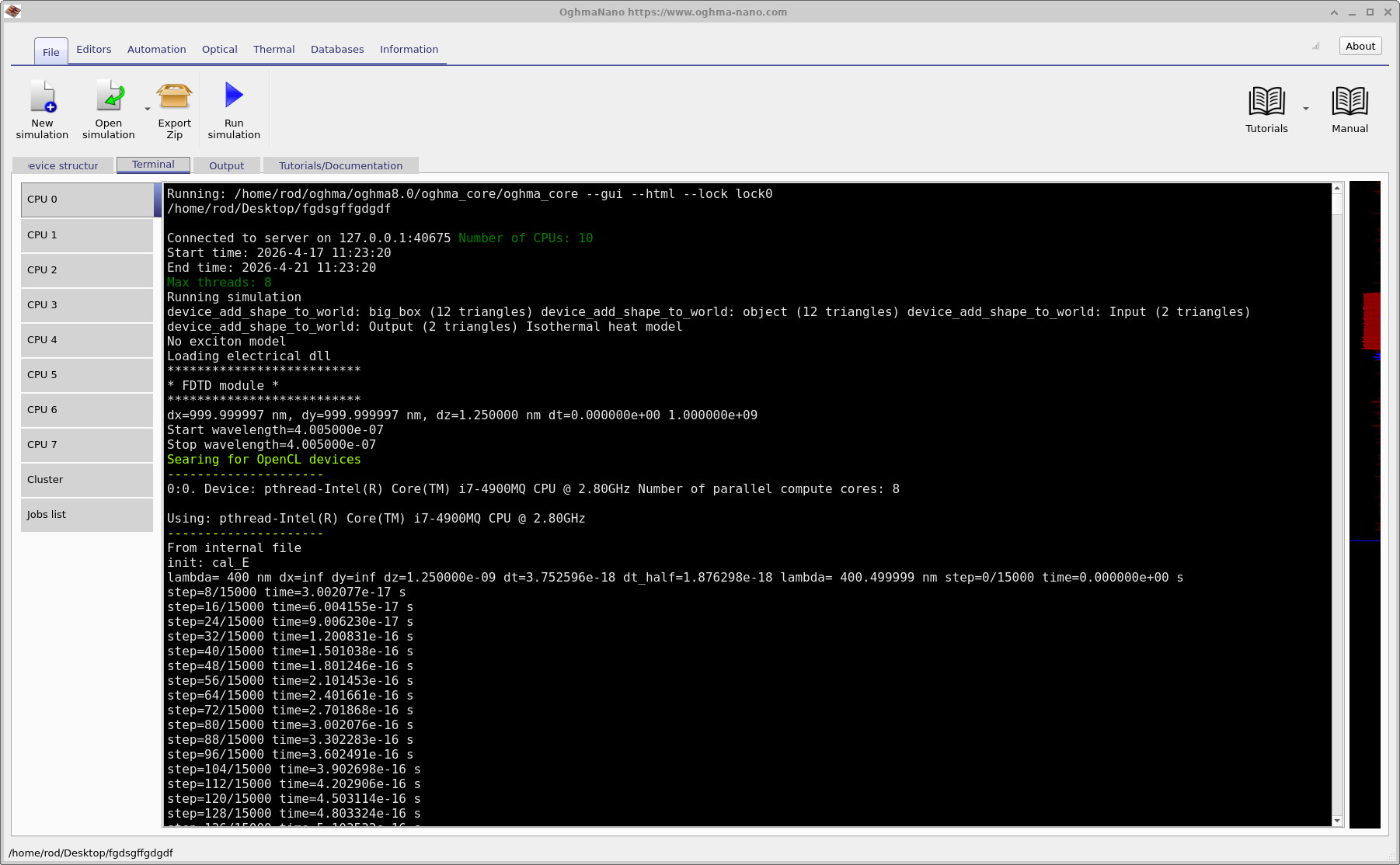
As the simulation runs, you can monitor its progress in the Terminal tab, shown in
??.
This displays information such as the timestep, wavelength range, and backend being used. Near the start of the run you will see a line saying Searching for OpenCL devices. These are hardware acceleration devices that can be used to speed up the simulation. If a suitable OpenCL device is found, as in the example shown in the figure, OghmaNano will use it automatically and run the simulation on the GPU rather than the CPU.
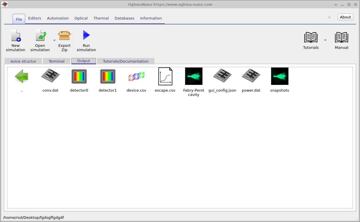
When the simulation has finished, switch to the Output tab, shown in
??.
Here you will find the data generated during the run. The key outputs for this tutorial are detector_0 and detector_1, which contain the signals recorded by the two detectors.
You can also open device to view the 3D geometry, and the snapshots/ directory to see how the electromagnetic fields evolve over time.
You should notice that this simulation runs very quickly. Because it is a 1D problem, typical run times are only a few seconds.
If the simulation is taking significantly longer than this, refer to the note above about saving the simulation on a fast local drive.
5. Viewing electric field snapshots
Open the snapshots/ output directory (from the Output tab) and double-click to launch the snapshot viewer.
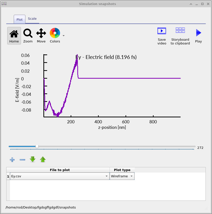
This allows you to view the simulation results as a function of time. Click the + button once to add a dataset, then select Ey. In this simulation the field is excited in the
y-direction, so this component gives the most direct view of the wave propagation.
You can then use the slider bar to step through time and observe how the field evolves. Three representative snapshots are shown in
??–
??.
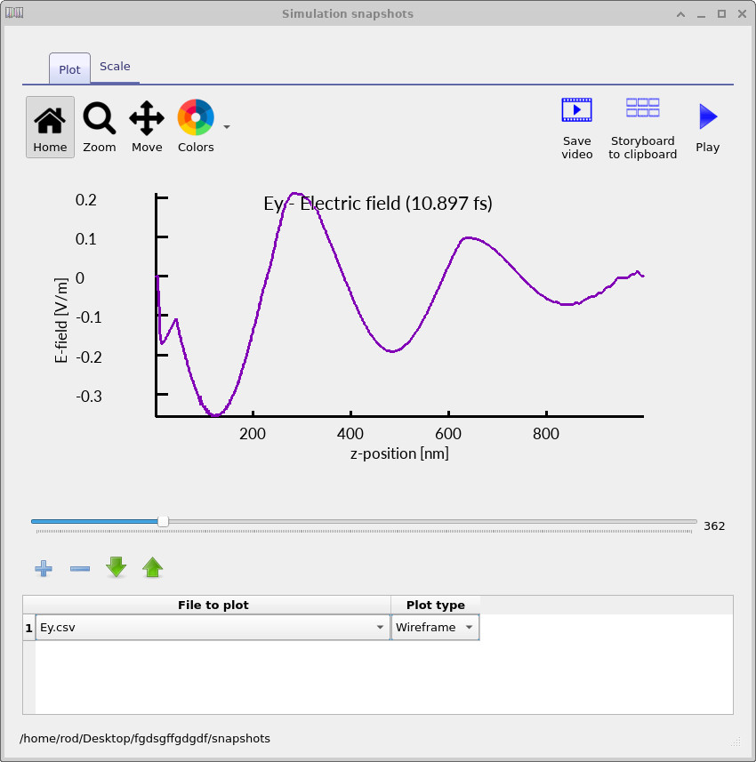
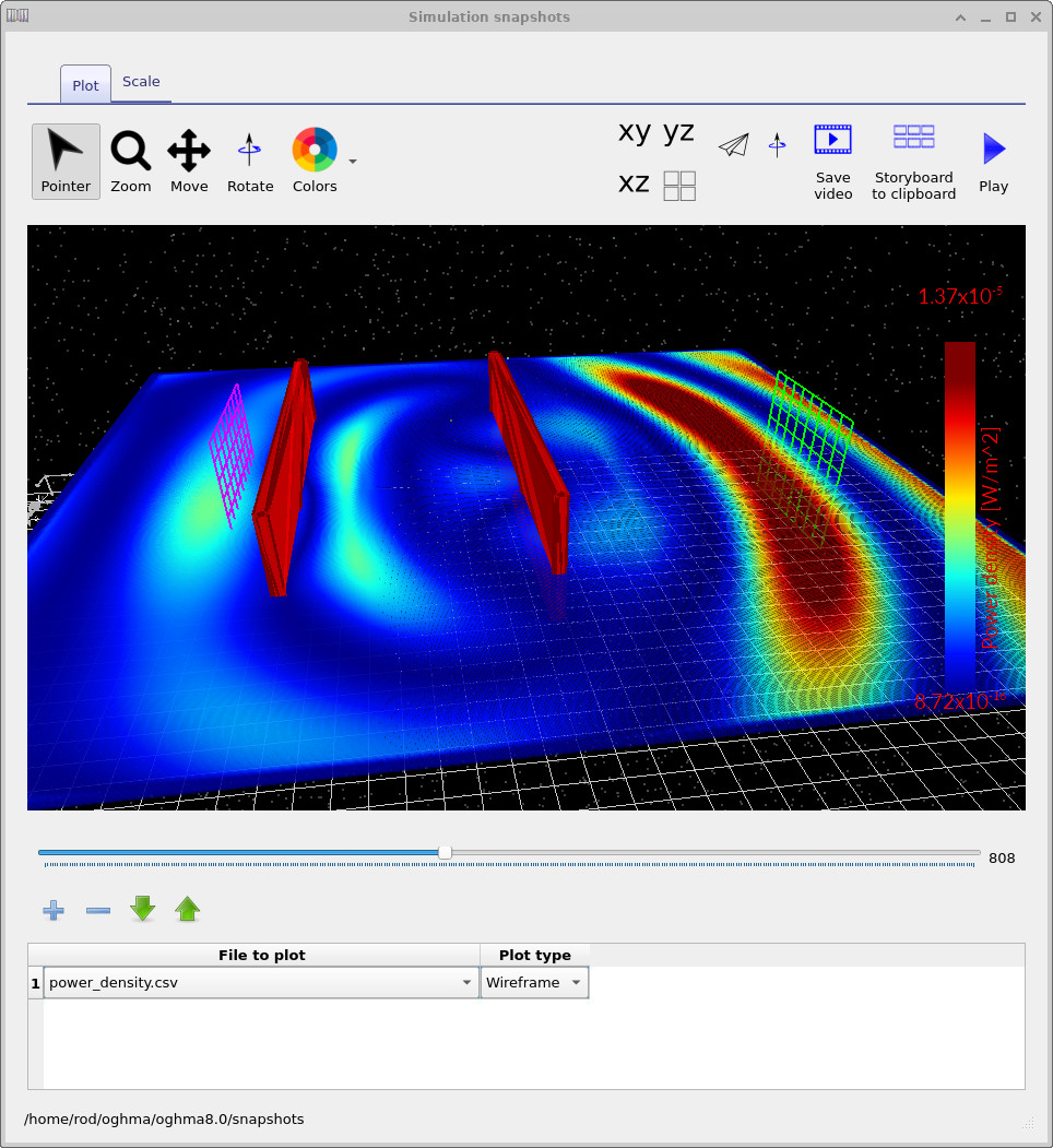
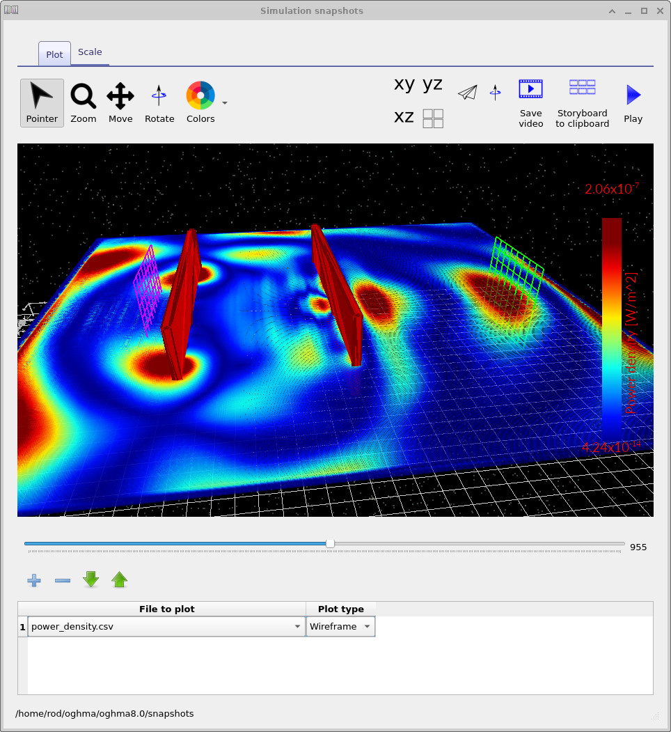
At early times (left panel), you can see the initial broadband pulse entering the structure. The field is still spatially localised, with a sharp leading edge corresponding to the injected excitation. As time progresses (middle panel), the pulse has interacted with the cavity region. The waveform becomes more structured and extended in space, indicating that multiple frequency components are propagating with different phases. This is a signature of partial reflection and interference within the structure.
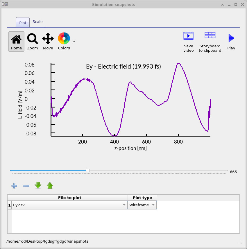
At later times (right panel), the field no longer resembles a single travelling pulse. Instead, it appears as a superposition of waves with different spatial frequencies. This behaviour arises because the cavity selectively enhances certain wavelengths while others are reflected or transmitted. The result is a complex interference pattern rather than a simple standing wave. It is worth noting that, because the simulation is excited with a broadband pulse and observed in the time domain, the cavity resonance does not appear immediately as a clean standing-wave mode. Instead, what you observe is the transient evolution toward resonance, where multiple reflections and interference gradually build up the frequency components that satisfy the cavity condition.
6. Viewing detector outputs
Returning to the Output tab (see
??),
you will see two detector folders, Detector0 and Detector1, which appear like small CCD sensor icons.
Detector0 is located on the source side of the cavity, while Detector1 is on the far side after the light has passed through the structure.
If you double-click on Detector0, you will see the contents shown in
??.
In this directory there are two files, lam_E.csv and power.csv.
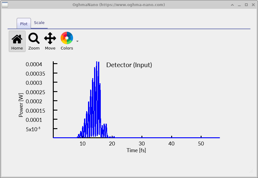
For now, open power.csv, which shows the power passing through the detector as a function of time. The result is shown in
??.
This is the power recorded at the input-side detector.
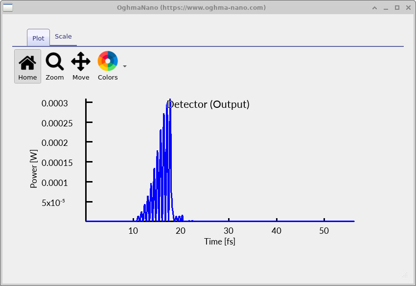
You can now repeat the same process for Detector1. Opening power.csv in that folder gives the result shown in
??.
In this case, the transmitted signal appears after a short delay corresponding to the time taken for the pulse to cross the cavity.
Compared to the input-side signal, the transmitted pulse is noticeably smoother and more regular. This reflects the fact that the cavity
preferentially transmits a narrower range of frequency components, while others are reflected. As a result, the output signal is effectively
a filtered version of the original broadband pulse.
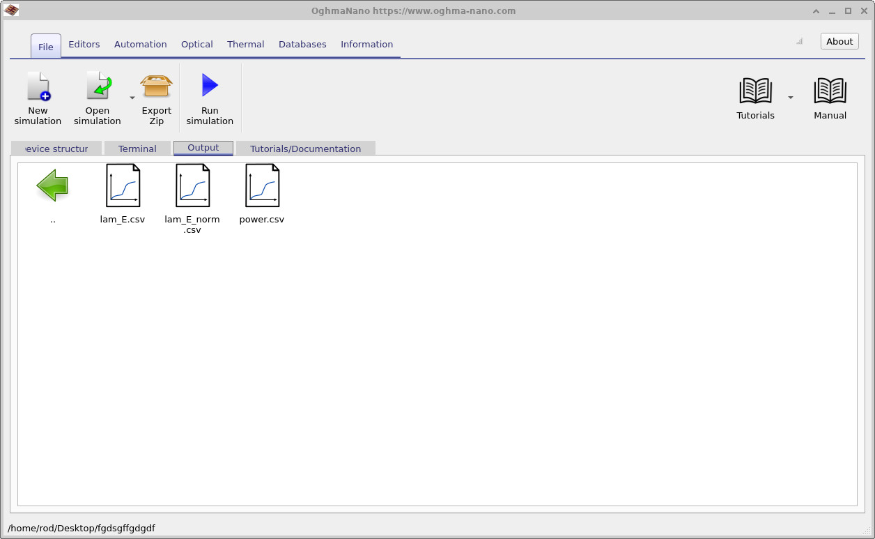
lam_E.csv and power.csv.
We can now move from the time-domain signals to the frequency-domain response. The signals shown previously can be
Fourier transformed to give the spectral content of the light passing through each detector. The frequency-domain data can be found in the file lam_E.csv inside both Detector0 and Detector1.
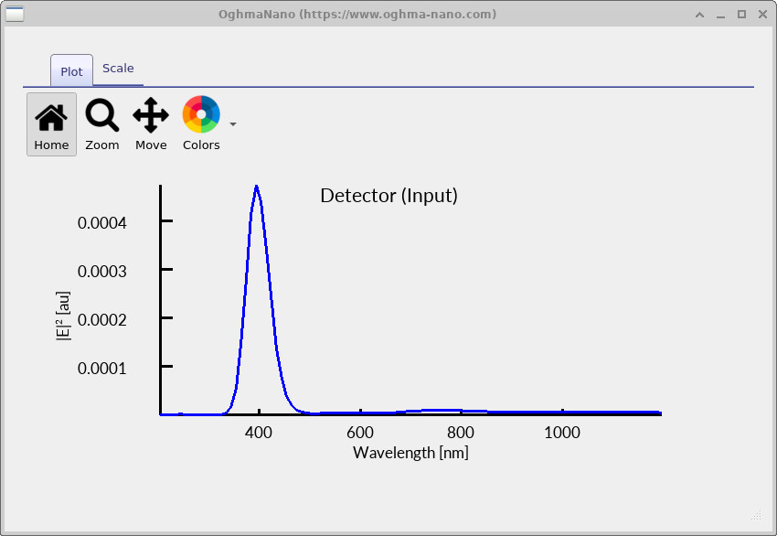
Input spectrum: The input-side spectrum is shown in ??. This is the spectrum recorded at the detector on the source side of the cavity. The dominant feature is a strong peak centred near 400 nm, corresponding to the main spectral content of the injected pulse. Because this detector is positioned before the cavity, the recorded spectrum is primarily the incident field, although it may also contain a small contribution from light reflected back from the structure. Away from the main peak, the signal becomes weak, and small features in these regions should not be over-interpreted.
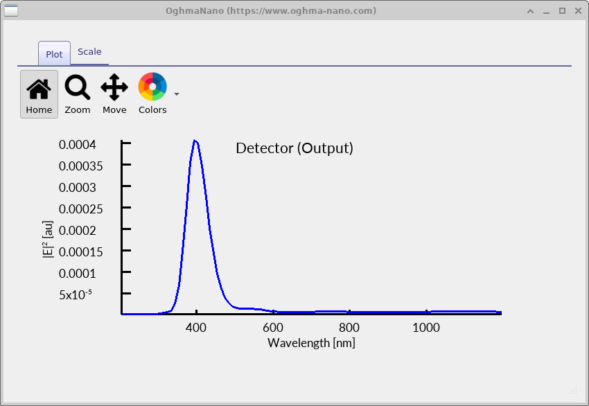
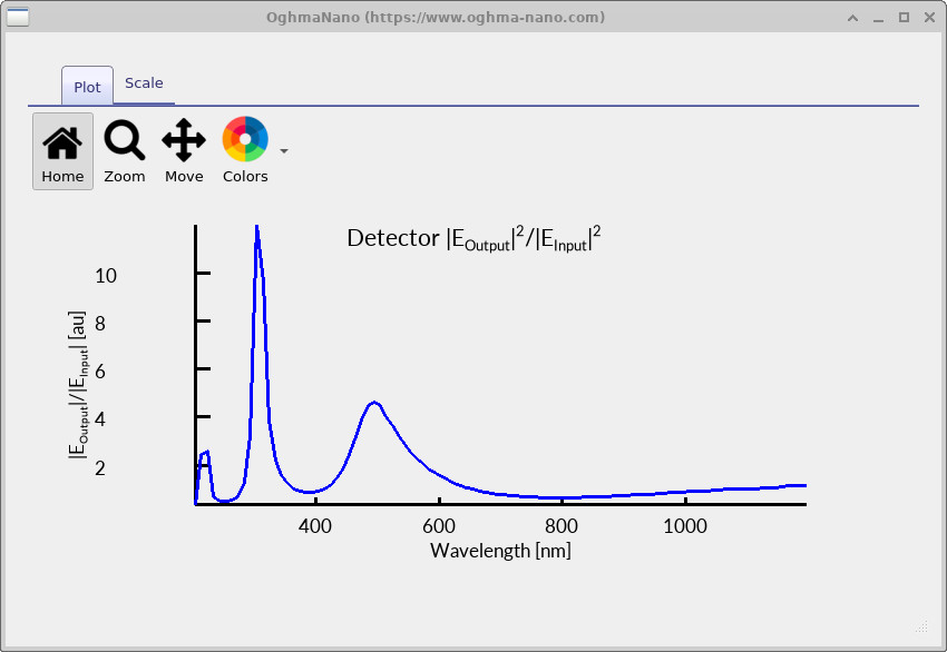
Output spectrum: The corresponding output-side spectrum is shown in ??. As with the input spectrum, the dominant feature is a strong peak near 400 nm, reflecting the primary excitation of the system. However, an additional feature is visible on the longer-wavelength side of this peak: a smaller shoulder around 500 nm. This feature arises from the response of the Fabry–Pérot cavity, which preferentially transmits certain wavelengths. Because the source is not centred on this resonance, the cavity-related feature appears only as a weaker secondary contribution rather than a dominant peak.
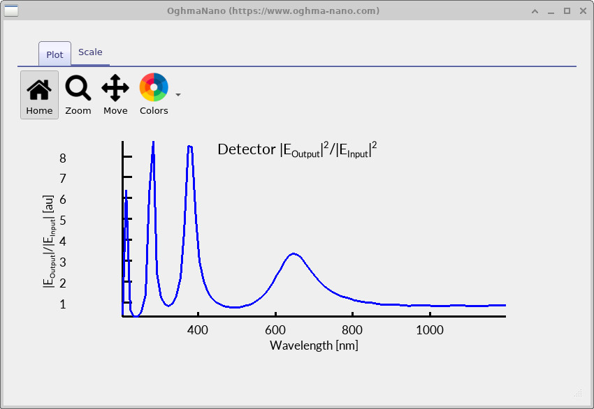
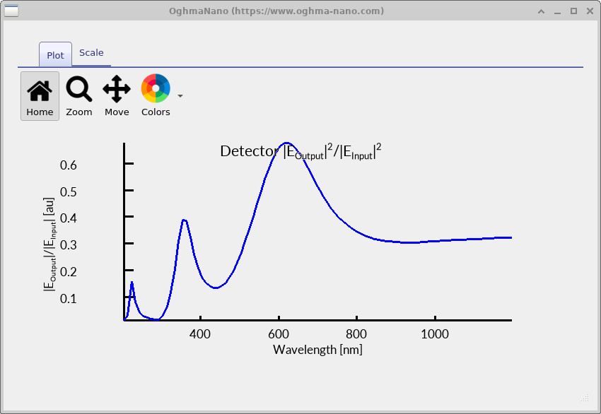
Input/output ratio: The spectra shown above are dominated by the spectral profile of the source, which makes it difficult to clearly see the effect of the cavity. To make the cavity response more visible, we need to remove, as far as possible, the influence of the source spectrum. We do this by dividing the output signal by the input signal, effectively normalising the transmitted field by the incident field. Since power is proportional to \(|E|^2\), this gives an approximate transmission function of the structure: \(T(\lambda) = \frac{|E_{\mathrm{output}}(\lambda)|^2}{|E_{\mathrm{input}}(\lambda)|^2}\). The result is shown in ??.
This procedure does not perfectly remove the source contribution, but it significantly reduces its influence. As a result, features associated with the cavity become much more apparent. In particular, the resonance around 500 nm, which appears only as a weak shoulder in the raw output spectrum, is now clearly enhanced in the normalised result. It should be noted that where the input signal is very small, the ratio can become large and noisy. These features are not physical resonances, but arise from dividing by a small number. For a cleaner transmission spectrum, a separate reference simulation without the cavity can be used for normalisation, but this is not required to observe the main effect here.
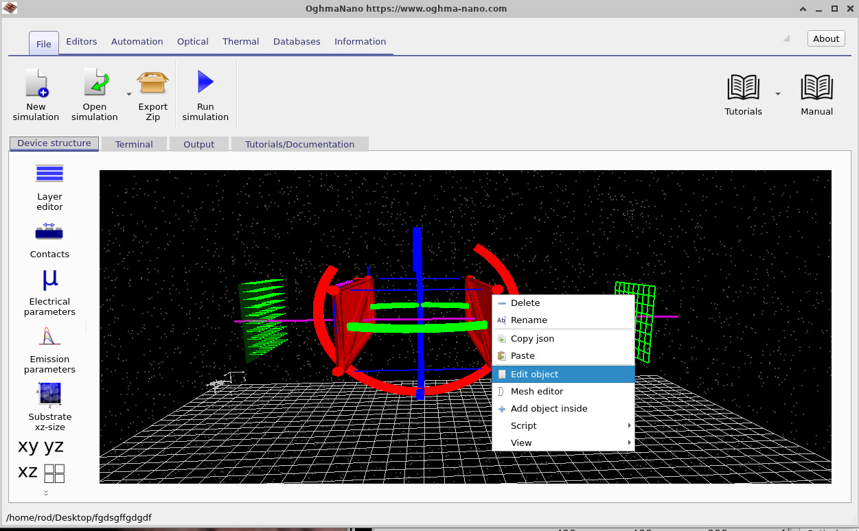
7. Experimenting with the cavity dimensions
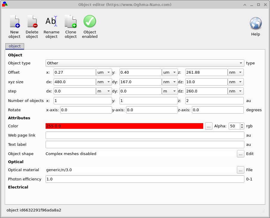
To explore how the Fabry–Pérot behaviour depends on its structure, right-click on one of the cavity mirrors and select Edit object, as shown in ??. This opens the object editor, where the geometry of the cavity can be controlled, as shown in ??. In this simulation, the cavity is formed by two thin mirrors, each 10 nm thick, separated by a gap of 250 nm. Rather than defining two independent objects, OghmaNano uses a replication feature: a single object is defined and then repeated along a chosen direction. In this case, the mirror is duplicated along the z-axis. This is controlled by the Number of objects field, which is set to 2 in the z direction. The step parameter then defines the spacing between successive copies of the object. Here, the step in the z-direction is set to 260 nm. This value includes both the cavity spacing and the thickness of the first mirror. Since each mirror is 10 nm thick, the physical gap between the two mirrors is \(260 - 10 = 250\) nm, which defines the cavity length. This construction allows both mirrors to be controlled consistently by editing a single object.
To change the cavity length, modify the z-step from 260 nm to 360 nm in the object editor. This increases the mirror-to-mirror spacing from 250 nm to 350 nm. After applying this change, the structure should appear as shown in ??, where the cavity region is visibly larger. The resonant wavelengths of a Fabry–Pérot cavity are determined by the round-trip phase condition, \[ 2 n L = m \lambda, \] where \(n\) is the refractive index inside the cavity, \(L\) is the cavity length, and \(m\) is an integer mode number. Rearranging this gives \[ \lambda = \frac{2 n L}{m}. \]
In the original structure, with \(L = 250\) nm and \(n \approx 1\), the fundamental mode (\(m=1\)) occurs at \[ \lambda \approx 2 \times 1 \times 250 = 500\ \text{nm}. \] After increasing the cavity length to \(L = 350\) nm, the corresponding wavelength becomes \[ \lambda \approx 2 \times 1 \times 350 = 700\ \text{nm}. \] This is the expected shift in the dominant cavity resonance.
Now rerun the simulation and inspect the output spectrum from Detector1. The result is shown in ??. You should observe that the main cavity-related feature has shifted from around 500 nm to closer to 700 nm, in agreement with the simple model above.
In addition to the main resonance, you will also notice the presence of other, weaker modes. These correspond to higher-order solutions of the Fabry–Pérot condition (\(m = 2, 3, \dots\)). For example, when \(m=2\), the wavelength is approximately \(\lambda = 2 n L / 2 = nL\), giving a shorter-wavelength mode. Because the excitation is broadband, multiple values of \(m\) can be weakly excited, leading to several peaks in the spectrum. However, their strength depends on how well they overlap with the spectral content of the source and how efficiently they couple through the mirrors.
9. Extending to 2D
So far, we have considered a one-dimensional Fabry–Pérot cavity, where the fields vary only along the propagation direction. One of the strengths of the Finite-Difference Time-Domain (FDTD) method is that it can be extended naturally to higher dimensions. In this section, we extend the simulation to two dimensions and observe how the field behaviour changes.
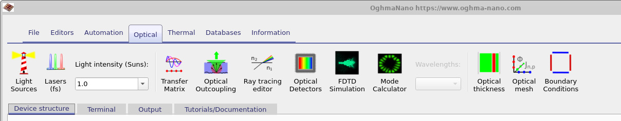
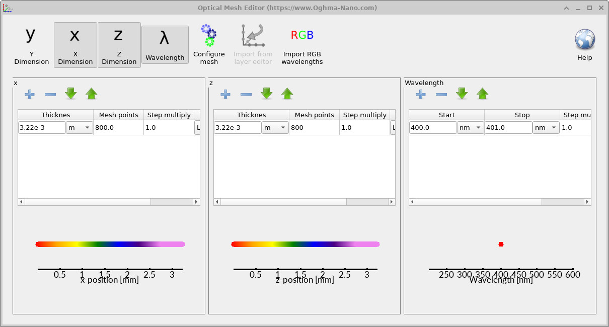
To do this, open the Optical ribbon (??) and launch the optical mesh editor. In the mesh editor (??), enable the x dimension so that the simulation solves for variation in both x and z. After applying this change, close the editor and rerun the simulation.
It should be noted that enabling an additional spatial dimension significantly increases the computational cost. The runtime can increase by up to an order of magnitude (typically up to 10× longer), because the number of grid points and field updates grows rapidly with dimensionality. This is a general feature of FDTD: increasing physical realism comes at the cost of increased computational effort.
After the simulation has completed, open the snapshots/ directory. Example results are shown in
??–
??.
Using the slider, you can step through time and observe how the wave propagates from the source,
spreads laterally, and interacts with the cavity before reaching the detector.
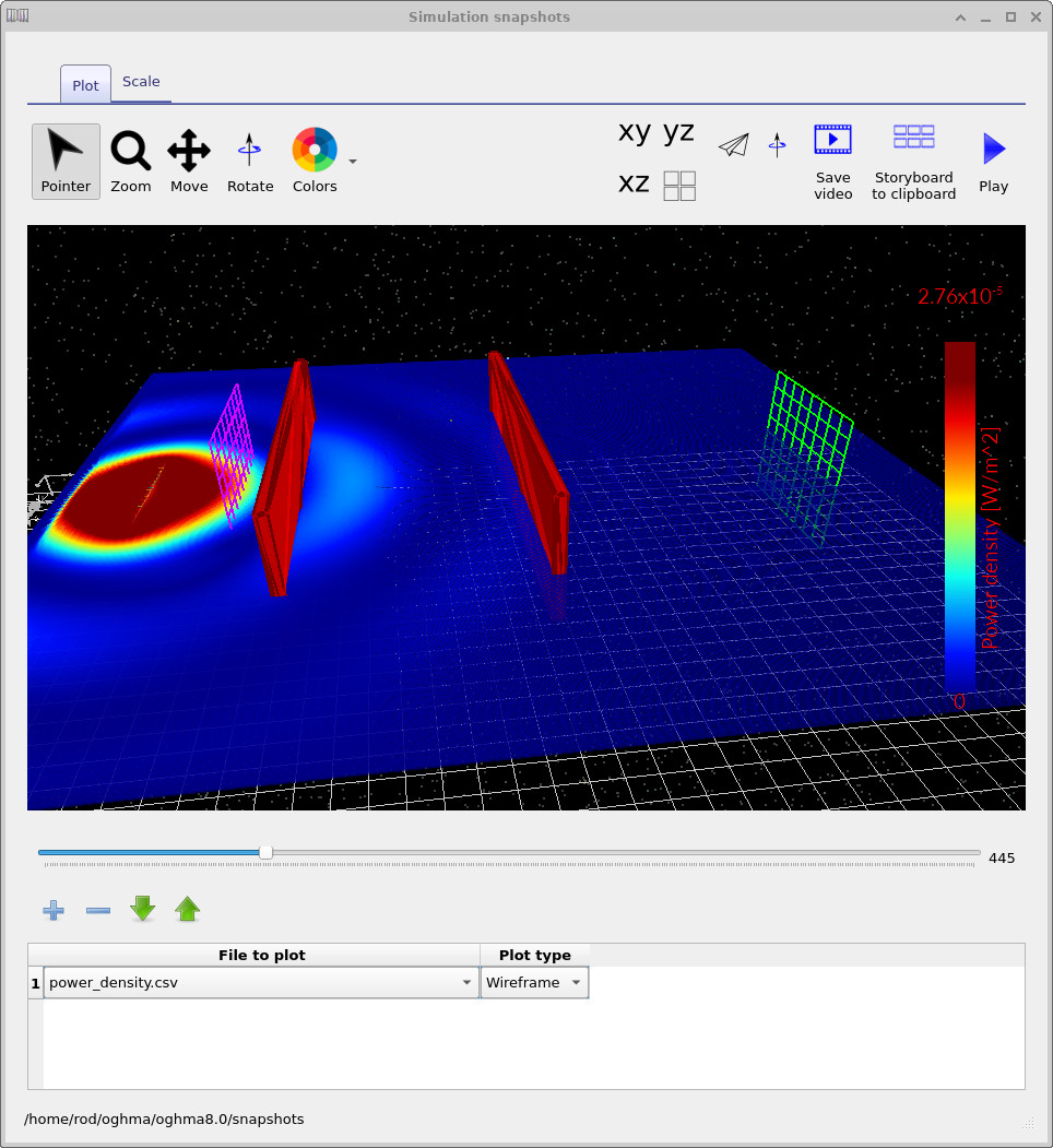
In contrast to the 1D case, the wavefront is no longer planar. Instead, it spreads out laterally, producing curved wavefronts and complex interference patterns. This means that light can travel through the cavity along multiple paths, not just directly between the two mirrors. As a result, the effective optical path length is no longer simply the geometric cavity length.
In 1D, the resonance condition is
\(2nL = m\lambda\)
However, in 2D the wave can propagate at an angle. If a ray travels at an angle \(\theta\) to the normal, the path length becomes
\(L_{\mathrm{eff}} = \frac{L}{\cos\theta}\)
and the resonance condition is modified to
\(2n \frac{L}{\cos\theta} = m\lambda\)
Because \(\cos\theta < 1\), the effective cavity length is larger than the physical length. This shifts the resonance to longer wavelengths, which explains why the peak in the 2D simulation appears around 600 nm rather than the value predicted by the simple 1D model (??).
This highlights an important result: while 1D simulations capture the basic Fabry–Pérot physics, higher-dimensional simulations introduce additional effects such as angular propagation, diffraction, and spatial mode structure. These effects are essential for understanding real optical systems, where light rarely propagates purely in one dimension.