FDTD optical detectors

1. Introduction

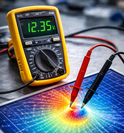
Digital voltmeter measuring an electric potential field, illustrating how a detector samples a field at a given location — A voltmeter measuring a potential field: detectors play a similar role in FDTD by sampling the electromagnetic field.

In FDTD simulations, optical detectors act like virtual measurement probes placed inside the simulation domain. A useful way to think about this is as a voltmeter, shown in ??: just as a voltmeter measures the electric potential at a specific point, an FDTD detector measures the electromagnetic field at a given location as a function of time.

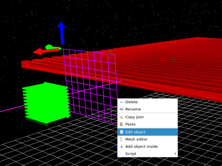
In practice, the detector samples the electric and magnetic fields at the grid points where it intersects the FDTD mesh. In a one-dimensional simulation, this corresponds to measuring the field along a line as the wave passes through it. In higher dimensions, the detector becomes a surface that records the spatial distribution of the field across its area. Visually, these detectors appear as grid-like planes in the simulation, as shown in ??.

As the simulation runs, the detector records the time-dependent field at its location. In addition, FDTD detectors can accumulate frequency-domain information directly during the simulation, allowing spectra to be obtained without performing a separate Fourier transform.

Optical detectors are described in more detail in the optical detectors section. Here, we focus specifically on their use in FDTD simulations.

2. Detector configuration

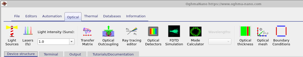
Detectors can be accessed from the Optical ribbon, as shown in ??, or by right-clicking on a detector object in the 3D view and selecting Edit object, as shown in ??.

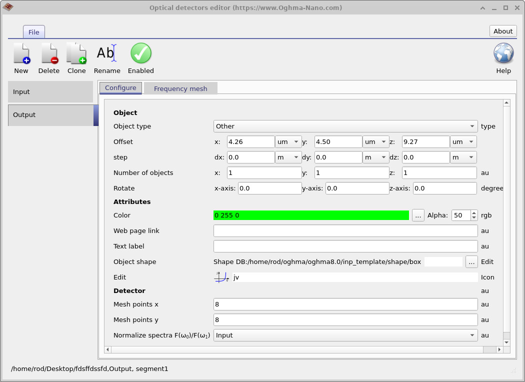
The detector configuration window is shown in ??. Each simulation may contain multiple detectors (for example, an input and output detector).

The Configure tab defines the detector geometry and position. While spatial mesh resolution is less critical in 1D FDTD simulations, an important setting is the normalised spectra option. This allows one detector to be normalised with respect to another. For example, an output detector can be normalised by an input detector to obtain a transmission spectrum.

Right-click menu on a detector in the 3D view showing the Edit object option — Detectors can also be accessed by right-clicking and selecting *Edit object*.

Optical ribbon in OghmaNano showing the Optical Detectors button used to open the detector editor — Opening the *Optical Detectors Editor* from the *Optical* ribbon.

Optical detectors editor showing detector list, geometry configuration, and normalisation options between detectors — Detector configuration panel showing geometry, position, and normalisation options.

Frequency mesh tab defining wavelength range and sampling points for FDTD spectral accumulation — Frequency mesh tab used to define the wavelength range for FDTD accumulators.

3. FDTD frequency-domain accumulators

In FDTD simulations, detectors can compute frequency-domain information directly during the simulation by accumulating the field response over time. Rather than storing the full time-dependent signal, the detector builds up the spectral content as the fields evolve.

At each timestep \(t_n = n\Delta t\), the detector updates a complex accumulator for each angular frequency \(\omega\):

\(E(\omega) = \sum_{n=0}^{N} E(t_n)\,e^{-i\omega t_n}\,\Delta t\)

where \(E(t_n)\) is the electric field recorded at the detector at timestep \(t_n\), and \(\Delta t\) is the simulation timestep. This expression is the discrete form of the Fourier transform, evaluated incrementally as the simulation progresses, with each timestep contributing a small complex phasor to the running sum.

Physically, this corresponds to projecting the time-domain field onto sinusoidal components \(e^{-i\omega t}\). Field components oscillating at frequency \(\omega\) add coherently over time, while other components average out, allowing the detector to isolate the spectral content of the signal.

In practice, the detector maintains a separate accumulator for each frequency defined in the simulation. As the wave passes through the detector, the spectrum is built up continuously without storing the full time-domain signal.

This approach has several important advantages:

No need to store large time-domain datasets
Reduced numerical noise compared to FFT post-processing
Direct access to spectral quantities such as transmission and reflection
Efficient accumulation over long simulation times

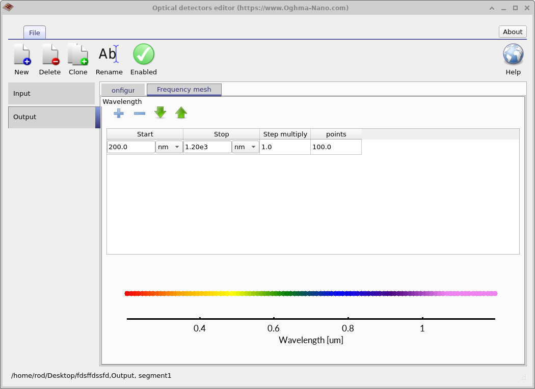
The frequencies (or wavelengths) at which the accumulation is performed are defined in the Frequency mesh tab shown in ??.

4. Detector outputs

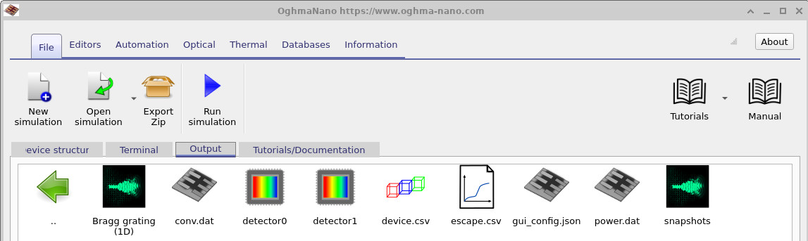
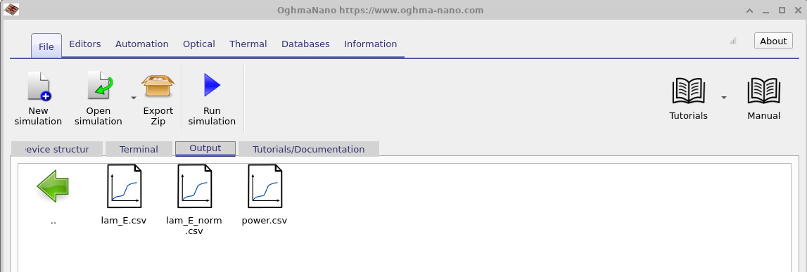
Output tab in OghmaNano showing a detector represented as a CCD-style icon — Detector output shown as a CCD-style icon in the output tab.

Expanded detector output folder showing files such as spectra and time-domain data — Files generated by the detector after the simulation.

After running the simulation, detector outputs appear as a small CCD-style icon in the output tab (??). Double-clicking this icon reveals the output files shown in ??.

Raw electric field spectrum versus wavelength obtained from FDTD frequency-domain accumulator — Raw electric field spectrum from the detector.

Normalised electric field spectrum showing transmission calculated by dividing output detector by input detector — Normalised spectrum showing transmission.

Time-domain power signal recorded by an FDTD detector showing pulse propagation through the simulation — Time-domain power recorded by the detector.

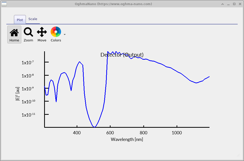
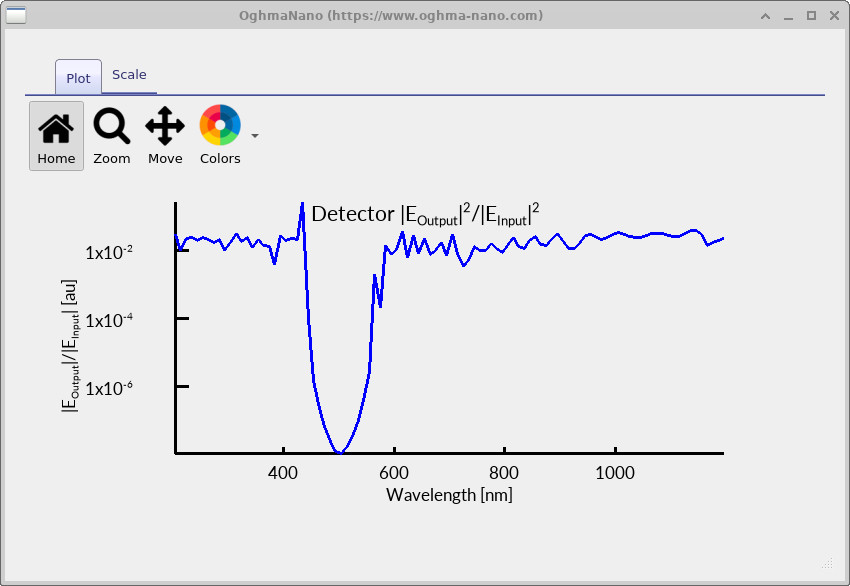
The files lam_E.csv and lam_E_norm.csv are generated directly from the frequency-domain accumulators. The first shows the raw electric field spectrum, while the second shows the normalised spectrum (for example, output divided by input).

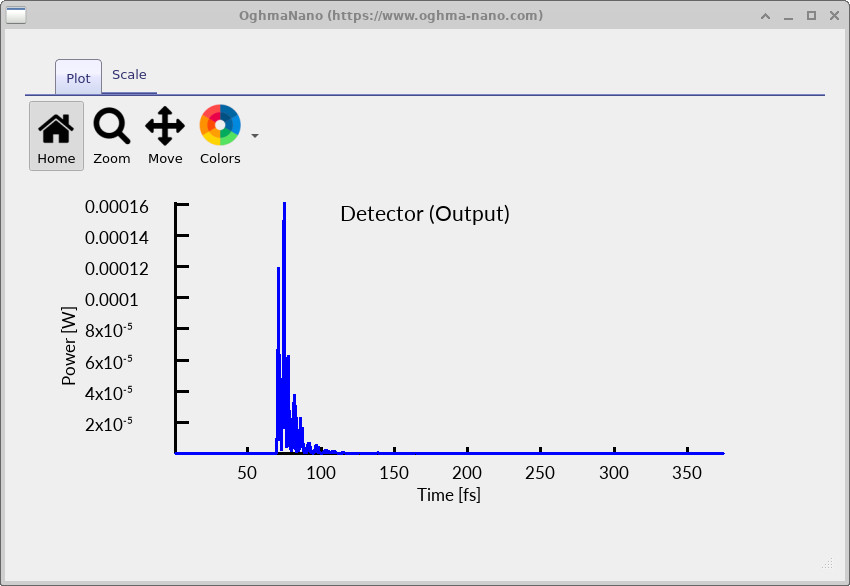
The file power.csv contains the time-domain signal recorded at the detector, as shown in ??.

It is important to note that the frequency-domain spectra are not obtained by applying an FFT to the time-domain signal. Instead, they are built directly during the simulation using the accumulators described above.