FDTD boundary conditions
1. Introduction
In finite-difference time-domain (FDTD) simulations, the boundary conditions define how electromagnetic fields behave at the outer limits of the computational domain. In physical terms, they determine what happens when a wave reaches the edge of the simulation cell. This is one of the most important aspects of an FDTD model because the numerical domain is always finite, whereas the physical problem often represents propagation in open space, repeated structures, or confined cavities. The role of the boundary condition is therefore to impose the correct mathematical continuation of the fields beyond the truncated mesh.
If a boundary is chosen poorly, waves reflect back into the mesh, interfere with the physical solution, and can produce strong standing-wave artefacts. In the worst case, energy becomes trapped inside the simulation volume and the calculated field distribution no longer represents the intended device. This is especially important in open photonic structures, scattering problems, radiating systems, and impulse-response calculations, where outgoing waves must leave the domain cleanly. Conversely, in periodic structures the correct behaviour is not absorption but repetition, and in some test problems it is desirable to fix the fields explicitly at the boundary. The choice of boundary condition must therefore match the physics of the model.
Mathematically, Maxwell’s curl equations are solved on a finite Yee grid. For a source-free isotropic region these may be written as
\[ \mu \frac{\partial \mathbf{H}}{\partial t} = - \nabla \times \mathbf{E}, \qquad \varepsilon \frac{\partial \mathbf{E}}{\partial t} + \sigma \mathbf{E} = \nabla \times \mathbf{H}. \]
The interior update equations follow directly from these relations, but at the outermost cells the stencil reaches beyond the stored mesh. The boundary condition provides the missing information required to complete the update. In practice this means that each outer face of the simulation box must be assigned a numerical rule which determines whether the tangential fields are fixed, absorbed, wrapped periodically, or attenuated through a matched absorbing layer.
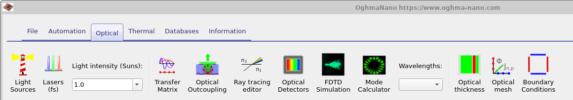
In OghmaNano, boundary conditions are configured from the Boundary Conditions button on the Optical ribbon (see Figure ??). The corresponding editor (see Figure ??) allows a different condition to be assigned to each outer face of the FDTD region. The available boundary types are Dirichlet, Mur ABC, Periodic, and PML.
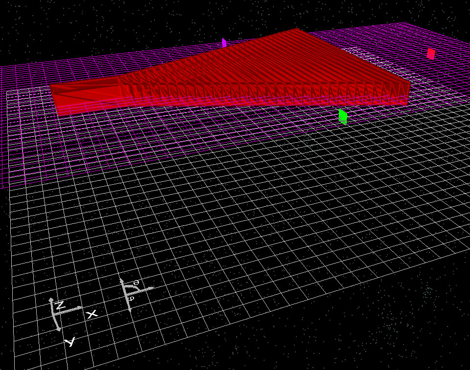
The six selectable boundaries correspond to the six faces of the Cartesian simulation box. In the default viewing configuration used by OghmaNano, \(y_0\) is the top face of the simulation region, \(y_1\) is the bottom face, \(x_0\) is the left face, \(x_1\) is the right face, \(z_0\) is the face closest to the user, and \(z_1\) is the face furthest from the user. The directional mapping is illustrated in Figure ??.
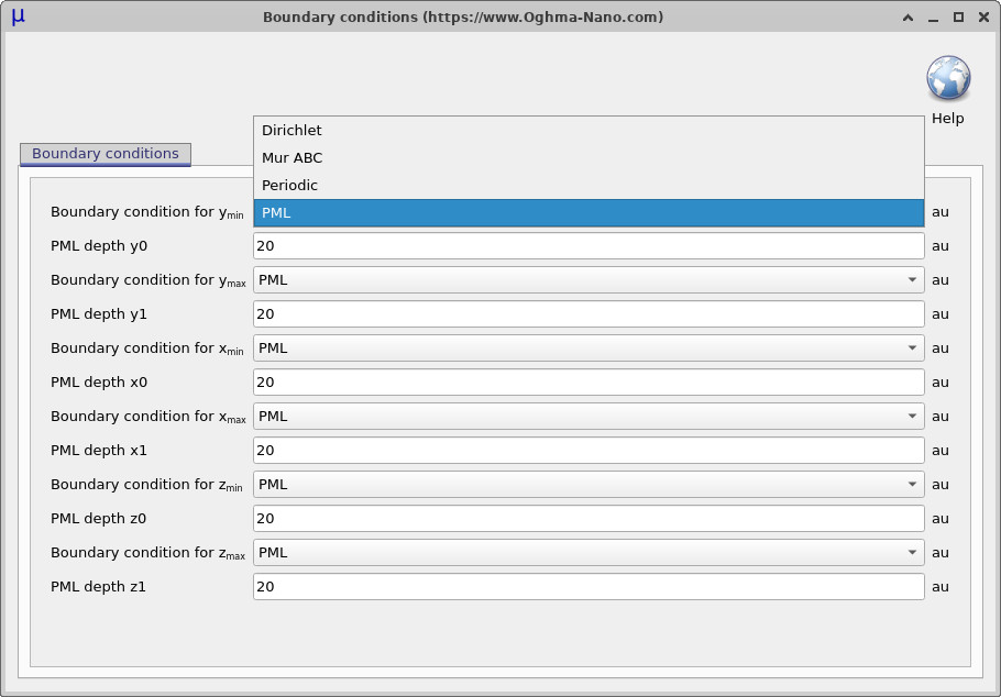
The boundary-condition editor assigns one rule to each of these six faces independently. This makes it possible to construct mixed domains, for example with periodic boundaries in the lateral directions and absorbing boundaries in the propagation direction, or with PML on all faces for radiation into free space. When PML is selected, an additional depth parameter is available for that face. This depth is given in mesh cells and determines how many outer FDTD layers are reserved for the absorbing medium.
2. Boundary-condition editor
The boundary-condition editor provides a separate control for the faces \(y_{\min}\), \(y_{\max}\), \(x_{\min}\), \(x_{\max}\), \(z_{\min}\), and \(z_{\max}\), corresponding respectively to \(y_0\), \(y_1\), \(x_0\), \(x_1\), \(z_0\), and \(z_1\) in the direction convention shown in Figure ??. For each face, the selected option determines how the tangential electric and magnetic fields are updated at the outer edge of the grid.
3. Dirichlet boundary condition
A Dirichlet boundary condition fixes the field on the boundary to a prescribed value. In the most common FDTD usage this value is zero, so the boundary enforces
\[ \mathbf{E}_{\mathrm{tan}} = 0 \qquad \text{on the selected face,} \]
The boundary therefore behaves as a perfectly reflecting wall for the electric field, and any outgoing wave is reflected back into the simulation region.
3. Mur ABC boundary condition
Mur absorbing boundary conditions are designed to reduce reflection by approximating the behaviour of an outward-travelling wave at the edge of the computational domain. The idea is to satisfy a one-way wave equation normal to the boundary so that energy leaving the grid continues to propagate outwards rather than reflecting back.
For a one-dimensional wave travelling in the \(+x\) direction, the exact outgoing-wave relation is
\[ \frac{\partial u}{\partial x} + \frac{1}{c}\frac{\partial u}{\partial t}=0. \]
Mur’s first-order absorbing boundary condition is obtained by discretising this equation on the FDTD mesh. On the left boundary, a standard form is
\[ u_0^{n+1} = u_1^{n} + \frac{c\Delta t-\Delta x}{c\Delta t+\Delta x} \left( u_1^{n+1}-u_0^{n} \right), \]
with an analogous expression on the opposite side. Here \(u_i^n\) denotes the field at spatial index \(i\) and time index \(n\), \(\Delta x\) is the mesh spacing, and \(\Delta t\) is the FDTD time step.
Mur absorbing boundary conditions are computationally inexpensive and require very little additional memory, which makes them attractive for lightweight simulations or exploratory calculations. They attempt to approximate an outgoing wave so that energy can leave the simulation domain rather than reflecting from the outer boundary.
Because the Mur condition is only an approximation, some reflection always remains. The accuracy deteriorates for oblique incidence, broadband pulses, and complex multi-dimensional scattering fields. Mur boundaries are therefore most appropriate for simple propagation problems where waves approach the boundary approximately normal to the surface and very high accuracy is not required.
For demanding optical simulations, radiating structures, or cases where waves strike the boundary from multiple angles, perfectly matched layers (PML) should be used instead. PML boundaries introduce an absorbing region that removes outgoing waves far more effectively and with significantly lower reflection than Mur conditions.
4. Periodic boundary condition
A periodic boundary condition identifies one face of the simulation region with the opposite face so that the field exiting one side re-enters through the other. This is appropriate when the physical structure repeats indefinitely in space and the computational cell represents a single unit cell of that repeating geometry.
In its simplest form, periodicity imposes
\[ \mathbf{E}(x+L_x,y,z,t)=\mathbf{E}(x,y,z,t), \qquad \mathbf{H}(x+L_x,y,z,t)=\mathbf{H}(x,y,z,t), \]
and similarly in the \(y\) or \(z\) directions when those boundaries are marked periodic. Numerically, the field values required just beyond one side of the domain are taken from the opposite side. Opposite faces must therefore be treated as a matched pair. Physically, this means the solution corresponds not to an isolated object, but to an infinite lattice of copies of the simulated cell.
Periodic boundaries are commonly used for structures that repeat in space, such as diffraction gratings, photonic crystals, metamaterial unit cells, and periodic waveguide geometries. By modelling only a single unit cell, the computational cost can be greatly reduced while still representing the behaviour of the full repeated structure, provided the source and geometry are consistent with the assumed periodicity.
With periodic boundaries, fields leaving one side of the simulation domain re-enter through the opposite side. Energy is therefore not absorbed but recirculated through the computational cell. Periodic boundaries should consequently not be used to represent open space. If periodic boundaries are applied on all faces of the simulation region, no energy can leave the domain and the total electromagnetic energy may accumulate over time. In many practical FDTD simulations, periodic boundaries are therefore applied in the transverse directions while absorbing boundaries such as PML are used in the propagation direction.
In the most general case, periodic fields may include a phase shift between adjacent cells. This is described by the Bloch condition
\[ \mathbf{E}(x+L_x,y,z,t)=\mathbf{E}(x,y,z,t)e^{ik_xL_x}, \]
with an analogous relation for the magnetic field. The standard periodic boundary implemented here corresponds to the special case \(k_x=0\), meaning the fields repeat identically across opposite faces of the simulation domain.
5. PML boundary condition
The perfectly matched layer (PML) is the standard high-performance absorbing boundary used in modern FDTD simulations. Its purpose is to remove outgoing electromagnetic waves with minimal reflection over a broad frequency range and for a wide spread of angles. Rather than imposing a one-step boundary formula at the outer edge, PML introduces an artificial absorbing medium surrounding the physical simulation region. Waves entering this layer experience attenuation without seeing a sharp impedance mismatch at the interface.
The defining idea is that the PML is matched to the interior medium at the entrance plane, so an incoming wave does not encounter a discontinuity that would itself generate reflection. Once inside the layer, the fields are damped exponentially. In continuous form this may be interpreted through a complex coordinate stretching, for example
\[ x \;\rightarrow\; \int_0^x s_x(\xi)\,d\xi, \qquad s_x(\xi)=\kappa_x(\xi)+\frac{\sigma_x(\xi)}{j\omega\varepsilon_0}, \]
with corresponding stretch factors in the other directions. Here \(\sigma_x\) is an artificial conductivity profile and \(\kappa_x\) is a scaling factor used in stretched-coordinate PML formulations. The effect is that propagating fields are attenuated as they traverse the layer while remaining approximately reflection-free at the interface with the physical domain.
In OghmaNano, selecting PML for a given face activates this absorbing layer on that side of the simulation region. The associated PML depth parameter sets the number of mesh cells allocated to the layer. A thicker PML generally provides stronger attenuation because the field has more distance over which to decay. If the PML is too thin, some energy can reach the outer truncation and reflect. If it is sufficiently thick, the outgoing field is damped to a negligible value before it reaches the outer edge.
A convenient way to understand the thickness dependence is to note that a field component inside an absorbing medium decays approximately as
\[ E(d)\sim E(0)\exp(-\alpha d), \]
where \(d\) is the distance travelled into the PML and \(\alpha\) is an effective attenuation coefficient set by the conductivity grading. Increasing the number of PML cells therefore reduces the residual amplitude reaching the exterior truncation. In practical terms, the PML depth should be large enough that reflections from the back of the layer are negligible compared with the physical signal of interest.
PML is usually the preferred boundary condition for open photonic and electromagnetic simulations, including waveguide radiation, scattering from isolated objects, antenna-like emission, and transient pulse propagation. It is far more robust than simple absorbing boundary conditions when fields strike the boundary obliquely or contain broad spectral content. For this reason, PML is the default choice in many FDTD models where waves are expected to leave the computational box.
Even with PML, good modelling practice remains important. The absorbing layer should not be placed too close to a strongly evanescent or highly resonant field region, because non-propagating near fields can interact with the absorbing material and alter the solution. In general, the physical structure should be separated from the PML by enough free space for the outgoing wavefront to form cleanly. Used in this way, PML provides the closest approximation in FDTD to an open, non-reflecting exterior domain.