How ray tracing works in optical systems

1. Introduction

OghmaNano showing 3D ray tracing through a Cooke Triplet lens — Full 3D ray tracing in OghmaNano. Rays are launched from a source, propagated through a multi-element optical system, and recorded on a detector plane.

Light bending by refraction at material interfaces — Refraction changes the direction of a ray when it crosses between materials with different refractive indices. In a complete optical system, repeated refraction through many surfaces determines the final image and throughput.

Ray tracing in optical systems is, in essence, the repeated application of geometric optical laws in three dimensions. A ray is defined by a position \(\mathbf{x}\), direction \(\mathbf{k}\), wavelength \(\lambda\), and optical power \(P\). As it propagates through a scene, it interacts with surfaces via refraction, reflection, absorption, and clipping.

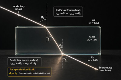
At each interface, the direction of the ray is determined by Snell’s law. In its scalar form:

\[ n_1 \sin(\theta_1) = n_2 \sin(\theta_2) \]

In practical simulations, ray tracing is performed in full three dimensions. This requires a vector formulation, where the incident direction \(\mathbf{k}_i\), surface normal \(\mathbf{n}\), and transmitted direction \(\mathbf{k}_t\) are explicitly computed. One common form is:

\[ \mathbf{k}_t = \frac{n_1}{n_2}\mathbf{k}_i + \left(\frac{n_1}{n_2}\cos\theta_i - \cos\theta_t\right)\mathbf{n} \]

where \(\cos\theta_i = -\mathbf{k}_i \cdot \mathbf{n}\) and \(\cos\theta_t\) follows from Snell’s law. This operation is applied at every interface in the system, allowing rays to be traced through arbitrarily complex assemblies of lenses, films, and structured surfaces (see ?? and ??).

In addition to direction changes, each interaction redistributes optical power between reflected and transmitted rays. This is governed by the Fresnel equations. For unpolarised light, a compact form is:

\[ R = \left|\frac{n_1 \cos\theta_i - n_2 \cos\theta_t}{n_1 \cos\theta_i + n_2 \cos\theta_t}\right|^2, \quad T = 1 - R \]

More generally, polarisation-dependent coefficients \(R_s, R_p\) and \(T_s, T_p\) can be used. These determine how optical power is partitioned at each boundary and are essential for predicting losses, throughput, and efficiency.

2. Naive brute-force ray tracing

In principle, ray tracing is therefore straightforward: propagate a ray, find the next intersection, apply Snell’s law and Fresnel relations, and continue. However, when simulating realistic optical systems (e.g. OLEDs, lenses, or light extraction from devices), one often needs to trace hundreds of thousands or millions of rays. The dominant cost is not the physics, but the search problem: determining which object a ray intersects first.

In a discretised scene, surfaces are typically represented as triangle meshes. A naive implementation would test a ray against every triangle in the scene. For a ray \(\mathbf{r}(t) = \mathbf{o} + t\mathbf{d}\) and triangle defined by vertices \(\mathbf{v}_0, \mathbf{v}_1, \mathbf{v}_2\), the intersection can be written in barycentric form:

\[ \mathbf{o} + t\mathbf{d} = \mathbf{v}_0 + u(\mathbf{v}_1 - \mathbf{v}_0) + v(\mathbf{v}_2 - \mathbf{v}_0), \quad u,v \ge 0,\; u+v \le 1 \]

Solving for \(t,u,v\) (e.g. via the Möller–Trumbore algorithm) determines whether the ray intersects the triangle. A brute-force search scales as \(\mathcal{O}(N)\) per ray for \(N\) triangles, which quickly becomes computationally prohibitive.

3. Faster ray tracing

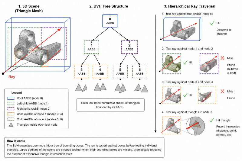
Bounding volume hierarchy (BVH) showing a ray intersecting bounding boxes before testing individual triangles — A bounding volume hierarchy (BVH) accelerates ray tracing by enclosing geometry in nested boxes. A ray is first tested against large bounding boxes; only if a box is hit does the algorithm descend into smaller boxes and eventually test individual triangles. Entire regions of the scene can be skipped if their bounding boxes are not intersected.

To address this, the scene is partitioned using spatial acceleration structures such as bounding volume hierarchies (BVH). The geometry is recursively subdivided into axis-aligned bounding boxes (AABBs), forming a tree structure. Each node contains a bounding volume enclosing a subset of triangles. Ray traversal then proceeds hierarchically: first intersect the bounding box, and only if it is hit, descend to child nodes.

This reduces the complexity of intersection tests from \(\mathcal{O}(N)\) toward \(\mathcal{O}(\log N)\) in practice, dramatically accelerating simulations. A schematic BVH structure is illustrated in ??.

Additional optimisations include multi-threading across CPU cores, early rejection of triangles behind the ray, and wavelength batching. Nevertheless, the core problem remains a search problem: efficiently identifying the first surface a ray encounters.

4. What does this mean for you as a user? (i.e. How do I make my simulation run faster)

When defining an optical scene, performance is strongly influenced by the number of geometric primitives. You should aim to minimise the triangle count while preserving physical accuracy. For example, when importing CAD models, unnecessary detail (e.g. bolts, threads, fine mechanical features) should be removed.

Each additional triangle increases the cost of ray–geometry intersection. This cost multiplies further when simulating multiple wavelengths or large ray ensembles. Therefore, unlike conventional CAD workflows, efficient optical modelling requires carefully simplified geometry that captures only optically relevant features.

In summary, ray tracing in optical systems consists of: the repeated application of Snell’s law in 3D, Fresnel reflection and transmission, and efficient search over scene geometry. Together, these form the foundation of physics-based optical simulation in OghmaNano.