FDTD vs Transfer Matrix Method (TMM): Choosing the Right Optical Simulation Method

🎯 Learning objectives

Understand the fundamental difference between FDTD and the transfer matrix method.
Learn when TMM is preferable to FDTD.
Understand the computational trade-offs between accuracy, dimensionality, and runtime.
Develop physical intuition for choosing the simplest valid optical model.

📦 Prerequisites

Basic familiarity with electromagnetic waves and optical interference.
Some understanding of multilayer optical structures is helpful.

⏱ Estimated time

Reading time: 15-20 min

Photon density map from transfer matrix simulation of a Fabry-Pérot cavity — Transfer matrix simulations directly reveal cavity resonances and standing-wave structure.

2D FDTD Fabry-Pérot cavity field distribution showing diffraction and interference — FDTD naturally captures diffraction, lateral propagation, and multidimensional interference.

1. Introduction

Both the transfer matrix method (TMM) and the finite-difference time-domain (FDTD) method are widely used for solving optical problems. However, despite both ultimately being based on Maxwell’s equations, they solve very different mathematical problems and are designed for different classes of physical systems.

One of the most common mistakes made by new users is to assume that the “most advanced” simulation method is always the best one. In practice, this is rarely true. In computational physics, the goal is usually not to solve the most complicated possible problem, but instead to solve the the simplest problem capable of accurately describing the physics of interest.

This is an important idea because computational cost grows extremely rapidly with dimensionality and model complexity. A carefully chosen simplified model can often produce results that are physically clearer, easier to interpret, and many orders of magnitude faster to compute.

The transfer matrix method is an excellent example of this principle. Rather than solving the full electromagnetic problem in space and time, TMM assumes that the structure is effectively one-dimensional and layered, as described in Derivation of the transfer matrix method. Under this approximation, the electromagnetic field inside each layer can be written analytically as a superposition of forward and backward travelling waves.

The result is that extremely complex interference problems can often be solved in milliseconds, with very high numerical accuracy, while still capturing the essential cavity physics, standing-wave behaviour, reflection spectra, transmission spectra, and multilayer interference effects.

FDTD, by contrast, solves Maxwell’s equations directly on a spatial grid as the electromagnetic fields evolve in time. A detailed mathematical derivation is given in FDTD derivations and mathematical background. This makes FDTD dramatically more general and much more physically complete, but also substantially more computationally expensive.

⚖️ Occam’s razor in optical simulation

When building optical simulations, it is often best to follow the principle of Occam’s razor: use the simplest model that accurately captures the physics. Simpler methods are usually faster, easier to interpret, and less prone to unnecessary numerical complexity. For layered optical structures, a one-dimensional transfer matrix model is often sufficient, while more complex methods such as FDTD become necessary only when effects like diffraction, scattering, or multidimensional propagation are important.

A classic example of this idea in physics is Einstein’s early model of heat capacity, which later led to Bose-Einstein statistics. Although the model neglected much of the microscopic complexity of real solids, it still captured the essential physics and provided deep physical insight. Good scientific models are often valuable not because they include every possible effect, but because they isolate the physics that matters most for the problem being studied.

2. The fundamental difference between TMM and FDTD

The key conceptual difference between the two methods is that TMM simplifies the physics before solving the equations, while FDTD attempts to solve the full electromagnetic problem directly.

In the transfer matrix method, the structure is assumed to consist of planar layers stacked along a single direction. Since the material properties vary only along one axis, Maxwell’s equations reduce to a much simpler one-dimensional wave problem.

This means that many difficult electromagnetic effects simply never appear in the mathematics. For example, standard one-dimensional TMM does not naturally include:

Diffraction
Lateral propagation
Curved wavefronts
Scattering from arbitrary geometries
Waveguide bends
Localized defects in two or three dimensions

This is not a weakness of the method. It is precisely the reason the method is so fast.

By removing unnecessary degrees of freedom, TMM focuses computational effort only on the physics relevant to layered optical systems. For thin-film optics, dielectric mirrors, Fabry-Pérot resonators, OLED stacks, solar-cell interference effects, and multilayer coatings, this approximation is often extremely accurate.

FDTD takes the opposite approach. Rather than simplifying the geometry analytically, space is divided into a numerical grid and Maxwell’s equations are solved directly throughout the simulation domain. The electromagnetic fields propagate through the structure naturally as a function of time.

Because the full field evolution is retained, FDTD can model diffraction, angled propagation, scattering, transient behaviour, higher-dimensional interference, waveguide modes, and arbitrary nanophotonic structures.

3. Comparing the physical insight provided by each method

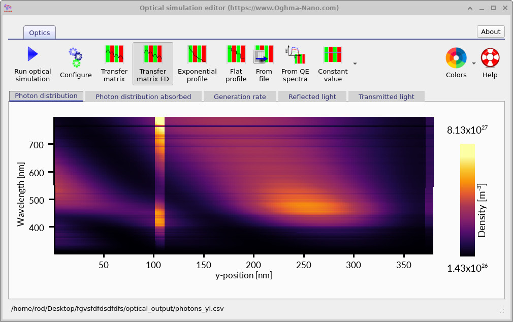
The transfer matrix method often provides extremely clean physical insight into resonant optical systems. For example, the Fabry-Pérot cavity photon-density map from the transfer matrix Fabry-Pérot cavity tutorial shown in ?? directly reveals the resonant wavelengths and standing-wave structure inside the cavity.

Because the problem is constrained to one dimension, the resonances are easy to interpret physically. The standing-wave modes appear clearly, the resonance wavelengths are sharply defined, and the connection between cavity length and resonance condition is immediately visible.

In many situations, this simplicity is highly desirable. The purpose of a simulation is often not merely to produce images, but to build physical understanding. Excessively complicated simulations can sometimes obscure the underlying physics rather than clarify it.

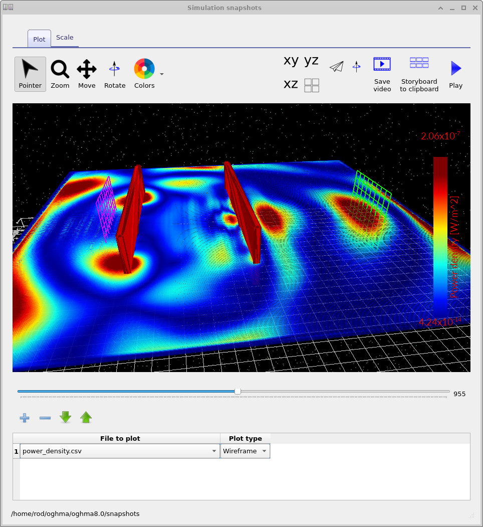
By contrast, the multidimensional FDTD simulation from the FDTD Fabry-Pérot cavity tutorial shown in ?? contains much richer spatial behaviour. Here the wave propagates in multiple dimensions, spreads laterally, diffracts, and forms complex interference patterns throughout the cavity region.

This additional realism is extremely important when the structure itself is genuinely multidimensional. However, it also means that the results can become substantially harder to interpret. The user must now distinguish between cavity resonances, diffraction effects, angular propagation, finite-size effects, transient behaviour, and numerical artefacts.

In other words, FDTD often provides more physics, but not always more useful physics.

4. Computational cost and scaling

One of the most important practical differences between the two methods is computational cost.

The transfer matrix method is extremely computationally efficient because it solves only a one-dimensional layered problem. Typical multilayer optical calculations complete in fractions of a second, even for structures containing many layers and broad wavelength sweeps.

In contrast, FDTD simulations scale very rapidly with dimensionality. If the spatial resolution is doubled, the number of grid points grows approximately as:

\(N\) in 1D
\(N^2\) in 2D
\(N^3\) in 3D

Additionally, the timestep must also decrease to satisfy numerical stability conditions. As a result, the total computational cost of FDTD can become enormous for large or high-resolution simulations.

This is why many realistic 3D FDTD simulations require:

GPU acceleration
Large memory capacity
Parallel computing
Long runtimes

Importantly, this does not mean FDTD is “bad”. It simply means that the method solves a much larger mathematical problem.

If the structure is fundamentally one-dimensional, using FDTD may provide very little additional physical accuracy while increasing the computational cost by several orders of magnitude.

5. When should you use the transfer matrix method?

In general, the transfer matrix method should be your first choice whenever the structure is approximately planar and layered.

TMM is particularly well suited for layered optical simulations such as optical filters, anti-reflective coatings, and Fabry-Pérot resonators. In general, TMM is especially well suited for:

Thin-film optics
Fabry-Pérot resonators
Optical coatings
Dielectric mirrors
Distributed Bragg reflectors (DBRs)
OLED optical modelling
Solar-cell interference calculations
Absorption calculations in layered stacks
Rapid parameter sweeps

TMM is also ideal when:

You need very fast simulations
You need to optimise many parameters
You want clean resonant spectra
You want simple physical interpretation
The structure is essentially one-dimensional

In many practical optical engineering problems, TMM can produce results that are almost indistinguishable from far more computationally expensive methods.

6. When should you use FDTD?

FDTD becomes important when the assumptions underlying TMM are no longer valid.

In particular, FDTD should be used when:

The geometry is genuinely two-dimensional or three-dimensional
Diffraction is important
The wave propagates at large angles
The structure contains bends or curves
The device contains isolated nanostructures
Scattering is important
Transient field evolution matters
You need full electromagnetic field distributions

Examples include:

In these systems, the simplifications used by TMM are no longer physically valid, so the additional computational effort of FDTD becomes necessary.

7. Final thoughts: solving the simplest valid problem

One of the most important skills in computational physics is learning how to choose the correct level of model complexity.

More complicated simulations are not automatically better simulations. In many cases, a simpler model can provide:

Clearer physical insight
Faster iteration
Easier debugging
Better parameter optimisation
More reliable interpretation

The transfer matrix method is powerful precisely because it removes unnecessary complexity from layered optical problems. It uses mathematical simplification intelligently, allowing the essential interference physics to be solved extremely efficiently.

FDTD becomes valuable when the neglected physics becomes important. At that point, the additional computational cost is justified because the simpler approximations are no longer adequate.

In practice, experienced researchers often use both methods together: TMM for rapid exploration and optimisation, followed by FDTD for detailed multidimensional validation and field analysis.

The goal is therefore not to choose the “most advanced” simulation technique, but instead to choose the method that most appropriately matches the underlying physics of the problem being solved.

🧩 Suggested exercises

Compare TMM and FDTD for the same Fabry-Pérot cavity.
Run both tutorials and compare the resonance positions and standing-wave structure.

Expected result
Both methods should predict similar resonance wavelengths for the 1D cavity. However, FDTD will additionally show transient behaviour, wave propagation, and multidimensional effects.
Increase the dimensionality of the FDTD simulation.
Extend the cavity from 1D to 2D and compare the resulting field patterns.

Expected result
The field will spread laterally, producing diffraction and angled propagation effects that cannot be captured using standard TMM.
Measure runtime scaling.
Compare the runtime of TMM and FDTD while increasing mesh resolution.

Expected result
FDTD runtime and memory usage increase rapidly with dimensionality and spatial resolution, while TMM remains extremely fast.